CS 5805 - Linear and nonlinear regression

a)Linear Regression

Index

What is Linear Regression
Types of Linear Regression
Training a Linear Regression Model
Finding the best fit line

What is Linear Regression

One of the simplest and most widely used machine learning algorithms is linear regression. It's a statistical technique for forecasting analysis. For continuous, real, or numerical variables like sales, salary, age, product price, etc., linear regression generates predictions.

Mathematically, we can represent a linear regression as:

y= a0+a1x+ ε

Y= Dependent Variable (Target Variable)
X= Independent Variable (predictor Variable)
a0= intercept of the line (Gives an additional degree of freedom)
a1 = Linear regression coefficient (scale factor to each input value).
ε = random error

The values for x and y variables are training datasets for Linear Regression model representation.

Types of Linear Regression

Simple Linear Regression
A linear regression algorithm is referred to as simple linear regression if it uses one independent variable to predict the value of a numerical dependent variable.

Y=β 0+β 1⋅X+ε
- Y is the dependent variable.
- X is the independent variable.
- β 0is the intercept (where the line crosses theY-axis).
- β 1 is the slop (the change in Y for a one-unitchange in X).
- ε is the error term, representing the variability in Y that is not explained by the linear relationship withX
Multiple Linear Regression
A type of linear regression algorithm known as multiple linear regression is used to predict the value of a numerical dependent variable by utilizing multiple independent variables.

Y=β 0+β 1⋅X 1 +β 2⋅X 2 +…+β n⋅X n+ε
- Y is the dependent variable.
- X 1,X 2,…,Xn are the independent variables
- β 0is the intercept
- β1,β 2,…,β nare the coefficients representing the impact of each independent variable.
- ε is the error term

Training a Linear Regression Model

Finding the values of the coefficients (β0,β1,...,βn) that minimize the sum of squared differences between the predicted and actual values in the training data is the first step in training a linear regression model.

Finding the best fit line

The best fit line should be found in order to minimize the error between the predicted and actual values. There will be the least error in the best fit line. We use the cost function to calculate the best values for a0 and a1 in order to find the best fit line because different weights or coefficients of lines (a0, a1) result in different regression lines.

Continuous random variable

A continuous random variable has two main characteristics:

Since there is no countable range of possible values, we integrate a function known as the probability density function to find the likelihood that a given value will fall within a given interval.

Common continuous distributions

Some examples of continuous distributions that are commonly used in statistics and probability theory can be found in the following table.

Name of the continuous distribution	Support
Uniform	All the real numbers in the interval [0,1]
Normal	The whole set of real numbers
Chi-square	The set of all non-negative real numbers

from sklearn.ensemble import GradientBoostingRegressor
import numpy as np
import pandas as pd
from sklearn.model_selection import train_test_split
from sklearn.metrics import mean_squared_error
from sklearn.metrics import mean_absolute_error
from sklearn.metrics import r2_score
from sklearn.datasets import load_iris
from sklearn.model_selection import train_test_split, GridSearchCV
import warnings
import seaborn as sns
import matplotlib.pyplot as plt
warnings.filterwarnings('ignore')

df = pd.read_csv('CarPrice_Assignment.csv')
df.head()

	car_ID	symboling	CarName	fueltype	aspiration	doornumber	carbody	drivewheel	enginelocation	wheelbase	...	enginesize	fuelsystem	boreratio	stroke	compressionratio	horsepower	peakrpm	citympg	highwaympg	price
0	1	3	alfa-romero giulia	gas	std	two	convertible	rwd	front	88.6	...	130	mpfi	3.47	2.68	9.0	111	5000	21	27	13495.0
1	2	3	alfa-romero stelvio	gas	std	two	convertible	rwd	front	88.6	...	130	mpfi	3.47	2.68	9.0	111	5000	21	27	16500.0
2	3	1	alfa-romero Quadrifoglio	gas	std	two	hatchback	rwd	front	94.5	...	152	mpfi	2.68	3.47	9.0	154	5000	19	26	16500.0
3	4	2	audi 100 ls	gas	std	four	sedan	fwd	front	99.8	...	109	mpfi	3.19	3.40	10.0	102	5500	24	30	13950.0
4	5	2	audi 100ls	gas	std	four	sedan	4wd	front	99.4	...	136	mpfi	3.19	3.40	8.0	115	5500	18	22	17450.0

5 rows × 26 columns

df.columns

Index(['car_ID', 'symboling', 'CarName', 'fueltype', 'aspiration',
       'doornumber', 'carbody', 'drivewheel', 'enginelocation', 'wheelbase',
       'carlength', 'carwidth', 'carheight', 'curbweight', 'enginetype',
       'cylindernumber', 'enginesize', 'fuelsystem', 'boreratio', 'stroke',
       'compressionratio', 'horsepower', 'peakrpm', 'citympg', 'highwaympg',
       'price'],
      dtype='object')

df.info()

<class 'pandas.core.frame.DataFrame'>
RangeIndex: 205 entries, 0 to 204
Data columns (total 26 columns):
 #   Column            Non-Null Count  Dtype  
---  ------            --------------  -----  
 0   car_ID            205 non-null    int64  
 1   symboling         205 non-null    int64  
 2   CarName           205 non-null    object 
 3   fueltype          205 non-null    object 
 4   aspiration        205 non-null    object 
 5   doornumber        205 non-null    object 
 6   carbody           205 non-null    object 
 7   drivewheel        205 non-null    object 
 8   enginelocation    205 non-null    object 
 9   wheelbase         205 non-null    float64
 10  carlength         205 non-null    float64
 11  carwidth          205 non-null    float64
 12  carheight         205 non-null    float64
 13  curbweight        205 non-null    int64  
 14  enginetype        205 non-null    object 
 15  cylindernumber    205 non-null    object 
 16  enginesize        205 non-null    int64  
 17  fuelsystem        205 non-null    object 
 18  boreratio         205 non-null    float64
 19  stroke            205 non-null    float64
 20  compressionratio  205 non-null    float64
 21  horsepower        205 non-null    int64  
 22  peakrpm           205 non-null    int64  
 23  citympg           205 non-null    int64  
 24  highwaympg        205 non-null    int64  
 25  price             205 non-null    float64
dtypes: float64(8), int64(8), object(10)
memory usage: 41.8+ KB

df.describe()

	car_ID	symboling	wheelbase	carlength	carwidth	carheight	curbweight	enginesize	boreratio	stroke	compressionratio	horsepower	peakrpm	citympg	highwaympg	price
count	205.000000	205.000000	205.000000	205.000000	205.000000	205.000000	205.000000	205.000000	205.000000	205.000000	205.000000	205.000000	205.000000	205.000000	205.000000	205.000000
mean	103.000000	0.834146	98.756585	174.049268	65.907805	53.724878	2555.565854	126.907317	3.329756	3.255415	10.142537	104.117073	5125.121951	25.219512	30.751220	13276.710571
std	59.322565	1.245307	6.021776	12.337289	2.145204	2.443522	520.680204	41.642693	0.270844	0.313597	3.972040	39.544167	476.985643	6.542142	6.886443	7988.852332
min	1.000000	-2.000000	86.600000	141.100000	60.300000	47.800000	1488.000000	61.000000	2.540000	2.070000	7.000000	48.000000	4150.000000	13.000000	16.000000	5118.000000
25%	52.000000	0.000000	94.500000	166.300000	64.100000	52.000000	2145.000000	97.000000	3.150000	3.110000	8.600000	70.000000	4800.000000	19.000000	25.000000	7788.000000
50%	103.000000	1.000000	97.000000	173.200000	65.500000	54.100000	2414.000000	120.000000	3.310000	3.290000	9.000000	95.000000	5200.000000	24.000000	30.000000	10295.000000
75%	154.000000	2.000000	102.400000	183.100000	66.900000	55.500000	2935.000000	141.000000	3.580000	3.410000	9.400000	116.000000	5500.000000	30.000000	34.000000	16503.000000
max	205.000000	3.000000	120.900000	208.100000	72.300000	59.800000	4066.000000	326.000000	3.940000	4.170000	23.000000	288.000000	6600.000000	49.000000	54.000000	45400.000000

df.shape

(205, 26)

df.isnull()

	car_ID	symboling	CarName	fueltype	aspiration	doornumber	carbody	drivewheel	enginelocation	wheelbase	...	enginesize	fuelsystem	boreratio	stroke	compressionratio	horsepower	peakrpm	citympg	highwaympg	price
0	False	False	False	False	False	False	False	False	False	False	...	False	False	False	False	False	False	False	False	False	False
1	False	False	False	False	False	False	False	False	False	False	...	False	False	False	False	False	False	False	False	False	False
2	False	False	False	False	False	False	False	False	False	False	...	False	False	False	False	False	False	False	False	False	False
3	False	False	False	False	False	False	False	False	False	False	...	False	False	False	False	False	False	False	False	False	False
4	False	False	False	False	False	False	False	False	False	False	...	False	False	False	False	False	False	False	False	False	False
...	...	...	...	...	...	...	...	...	...	...	...	...	...	...	...	...	...	...	...	...	...
200	False	False	False	False	False	False	False	False	False	False	...	False	False	False	False	False	False	False	False	False	False
201	False	False	False	False	False	False	False	False	False	False	...	False	False	False	False	False	False	False	False	False	False
202	False	False	False	False	False	False	False	False	False	False	...	False	False	False	False	False	False	False	False	False	False
203	False	False	False	False	False	False	False	False	False	False	...	False	False	False	False	False	False	False	False	False	False
204	False	False	False	False	False	False	False	False	False	False	...	False	False	False	False	False	False	False	False	False	False

205 rows × 26 columns

sns.heatmap(df.isnull(),yticklabels=False,cbar=False,cmap='viridis')

<Axes: >

df.dropna(inplace =True)
df.isnull().sum()

car_ID              0
symboling           0
CarName             0
fueltype            0
aspiration          0
doornumber          0
carbody             0
drivewheel          0
enginelocation      0
wheelbase           0
carlength           0
carwidth            0
carheight           0
curbweight          0
enginetype          0
cylindernumber      0
enginesize          0
fuelsystem          0
boreratio           0
stroke              0
compressionratio    0
horsepower          0
peakrpm             0
citympg             0
highwaympg          0
price               0
dtype: int64

df.duplicated().any()

False

df.describe(include=object)

	CarName	fueltype	aspiration	doornumber	carbody	drivewheel	enginelocation	enginetype	cylindernumber	fuelsystem
count	205	205	205	205	205	205	205	205	205	205
unique	147	2	2	2	5	3	2	7	7	8
top	toyota corona	gas	std	four	sedan	fwd	front	ohc	four	mpfi
freq	6	185	168	115	96	120	202	148	159	94

df = df.select_dtypes(include=['float64', 'int64'])
df.corr()

	car_ID	symboling	wheelbase	carlength	carwidth	carheight	curbweight	enginesize	boreratio	stroke	compressionratio	horsepower	peakrpm	citympg	highwaympg	price
car_ID	1.000000	-0.151621	0.129729	0.170636	0.052387	0.255960	0.071962	-0.033930	0.260064	-0.160824	0.150276	-0.015006	-0.203789	0.015940	0.011255	-0.109093
symboling	-0.151621	1.000000	-0.531954	-0.357612	-0.232919	-0.541038	-0.227691	-0.105790	-0.130051	-0.008735	-0.178515	0.070873	0.273606	-0.035823	0.034606	-0.079978
wheelbase	0.129729	-0.531954	1.000000	0.874587	0.795144	0.589435	0.776386	0.569329	0.488750	0.160959	0.249786	0.353294	-0.360469	-0.470414	-0.544082	0.577816
carlength	0.170636	-0.357612	0.874587	1.000000	0.841118	0.491029	0.877728	0.683360	0.606454	0.129533	0.158414	0.552623	-0.287242	-0.670909	-0.704662	0.682920
carwidth	0.052387	-0.232919	0.795144	0.841118	1.000000	0.279210	0.867032	0.735433	0.559150	0.182942	0.181129	0.640732	-0.220012	-0.642704	-0.677218	0.759325
carheight	0.255960	-0.541038	0.589435	0.491029	0.279210	1.000000	0.295572	0.067149	0.171071	-0.055307	0.261214	-0.108802	-0.320411	-0.048640	-0.107358	0.119336
curbweight	0.071962	-0.227691	0.776386	0.877728	0.867032	0.295572	1.000000	0.850594	0.648480	0.168790	0.151362	0.750739	-0.266243	-0.757414	-0.797465	0.835305
enginesize	-0.033930	-0.105790	0.569329	0.683360	0.735433	0.067149	0.850594	1.000000	0.583774	0.203129	0.028971	0.809769	-0.244660	-0.653658	-0.677470	0.874145
boreratio	0.260064	-0.130051	0.488750	0.606454	0.559150	0.171071	0.648480	0.583774	1.000000	-0.055909	0.005197	0.573677	-0.254976	-0.584532	-0.587012	0.553173
stroke	-0.160824	-0.008735	0.160959	0.129533	0.182942	-0.055307	0.168790	0.203129	-0.055909	1.000000	0.186110	0.080940	-0.067964	-0.042145	-0.043931	0.079443
compressionratio	0.150276	-0.178515	0.249786	0.158414	0.181129	0.261214	0.151362	0.028971	0.005197	0.186110	1.000000	-0.204326	-0.435741	0.324701	0.265201	0.067984
horsepower	-0.015006	0.070873	0.353294	0.552623	0.640732	-0.108802	0.750739	0.809769	0.573677	0.080940	-0.204326	1.000000	0.131073	-0.801456	-0.770544	0.808139
peakrpm	-0.203789	0.273606	-0.360469	-0.287242	-0.220012	-0.320411	-0.266243	-0.244660	-0.254976	-0.067964	-0.435741	0.131073	1.000000	-0.113544	-0.054275	-0.085267
citympg	0.015940	-0.035823	-0.470414	-0.670909	-0.642704	-0.048640	-0.757414	-0.653658	-0.584532	-0.042145	0.324701	-0.801456	-0.113544	1.000000	0.971337	-0.685751
highwaympg	0.011255	0.034606	-0.544082	-0.704662	-0.677218	-0.107358	-0.797465	-0.677470	-0.587012	-0.043931	0.265201	-0.770544	-0.054275	0.971337	1.000000	-0.697599
price	-0.109093	-0.079978	0.577816	0.682920	0.759325	0.119336	0.835305	0.874145	0.553173	0.079443	0.067984	0.808139	-0.085267	-0.685751	-0.697599	1.000000

correlation_matrix = df[['carlength', 'carwidth', 'curbweight']].corr()
plt.figure(figsize=(8, 6))
sns.heatmap(correlation_matrix,  cmap='coolwarm', center=0)
for i in range(len(correlation_matrix)):
    for j in range(len(correlation_matrix)):
        plt.text(j + 0.5, i + 0.5, f"{correlation_matrix.iloc[i, j]:.2f}", ha='center', va='center', fontsize=10)
plt.title('Correlation Matrix')
plt.show()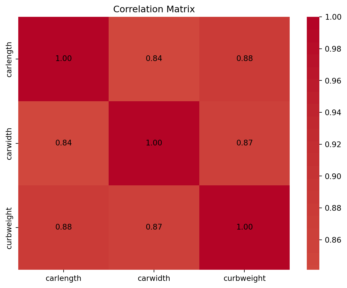

df = df.drop(['symboling', 'car_ID', ], axis=1)
print(df.head())

   wheelbase  carlength  carwidth  carheight  curbweight  enginesize  \
0       88.6      168.8      64.1       48.8        2548         130   
1       88.6      168.8      64.1       48.8        2548         130   
2       94.5      171.2      65.5       52.4        2823         152   
3       99.8      176.6      66.2       54.3        2337         109   
4       99.4      176.6      66.4       54.3        2824         136   

   boreratio  stroke  compressionratio  horsepower  peakrpm  citympg  \
0       3.47    2.68               9.0         111     5000       21   
1       3.47    2.68               9.0         111     5000       21   
2       2.68    3.47               9.0         154     5000       19   
3       3.19    3.40              10.0         102     5500       24   
4       3.19    3.40               8.0         115     5500       18   

   highwaympg    price  
0          27  13495.0  
1          27  16500.0  
2          26  16500.0  
3          30  13950.0  
4          22  17450.0

df.shape

(205, 14)

df.columns

Index(['wheelbase', 'carlength', 'carwidth', 'carheight', 'curbweight',
       'enginesize', 'boreratio', 'stroke', 'compressionratio', 'horsepower',
       'peakrpm', 'citympg', 'highwaympg', 'price'],
      dtype='object')

X = df.drop('price', axis=1)
y = df['price']

X.head()

	wheelbase	carlength	carwidth	carheight	curbweight	enginesize	boreratio	stroke	compressionratio	horsepower	peakrpm	citympg	highwaympg
0	88.6	168.8	64.1	48.8	2548	130	3.47	2.68	9.0	111	5000	21	27
1	88.6	168.8	64.1	48.8	2548	130	3.47	2.68	9.0	111	5000	21	27
2	94.5	171.2	65.5	52.4	2823	152	2.68	3.47	9.0	154	5000	19	26
3	99.8	176.6	66.2	54.3	2337	109	3.19	3.40	10.0	102	5500	24	30
4	99.4	176.6	66.4	54.3	2824	136	3.19	3.40	8.0	115	5500	18	22

0      13495.0
1      16500.0
2      16500.0
3      13950.0
4      17450.0
        ...   
200    16845.0
201    19045.0
202    21485.0
203    22470.0
204    22625.0
Name: price, Length: 205, dtype: float64

plt.figure(figsize=(8, 6))
sns.heatmap(df.corr(), cmap='coolwarm', fmt=".2f", linewidths=.5)
for i in range(len(df.corr())):
    for j in range(len(df.corr())):
        plt.text(j + 0.5, i + 0.5, f"{df.corr().iloc[i, j]:.2f}", ha='center', va='center', fontsize=10)
plt.title('Correlation Heatmap')
plt.show()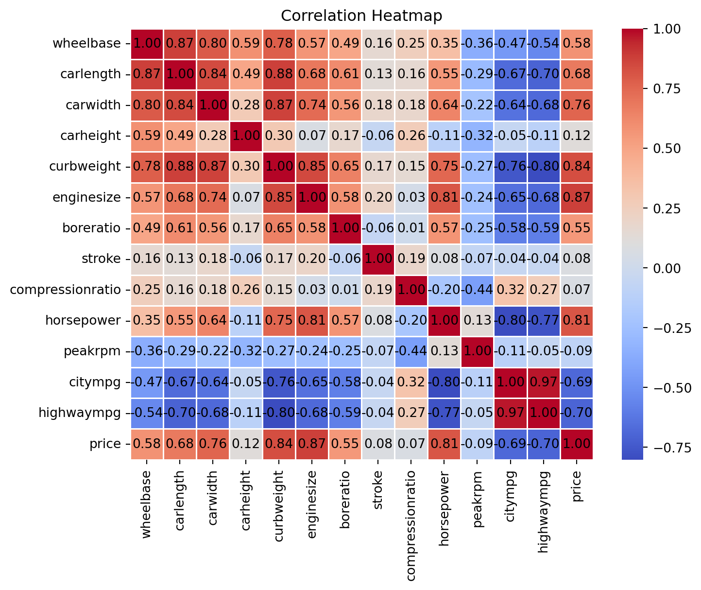

sns.pairplot(df)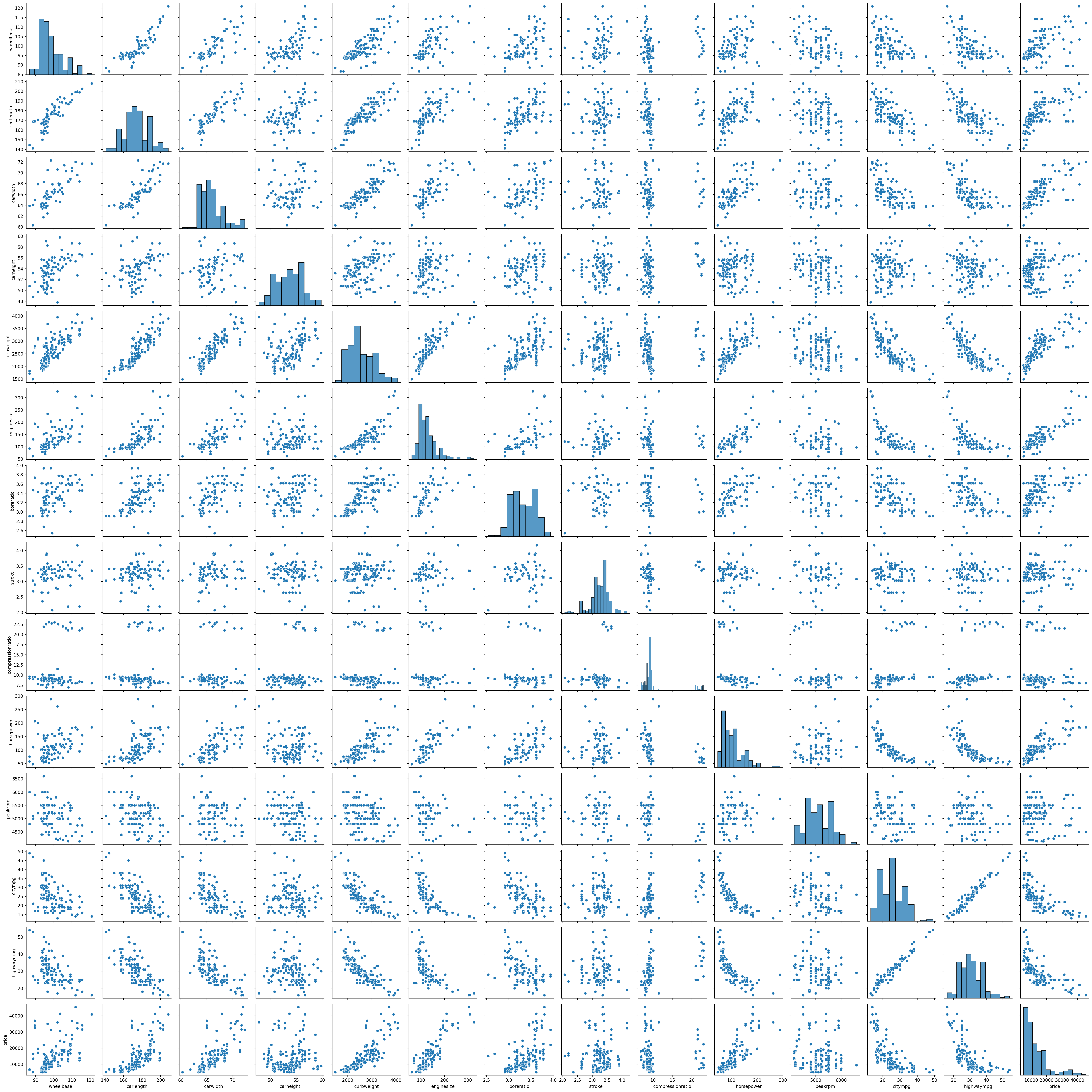

plt.figure(figsize=(8, 6))
sns.histplot(df['enginesize'], kde=True, color='skyblue')
plt.title('Distribution of Engine Size')
plt.show()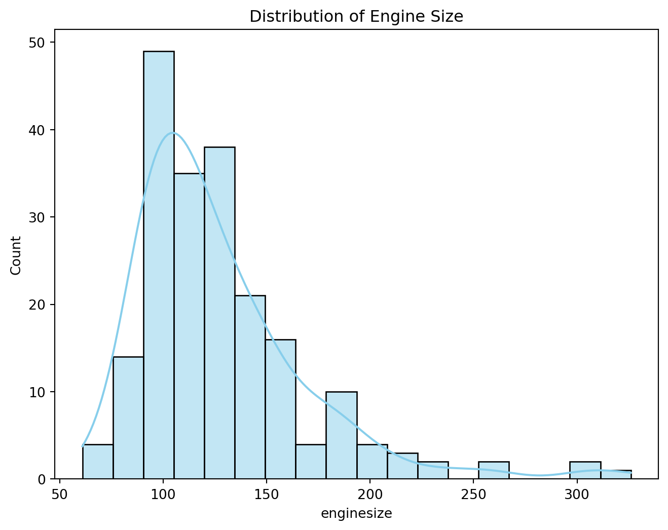

plt.figure(figsize=(8, 6))
sns.histplot(df['wheelbase'], kde=True)
plt.title('Distribution of Wheelbase')
plt.show()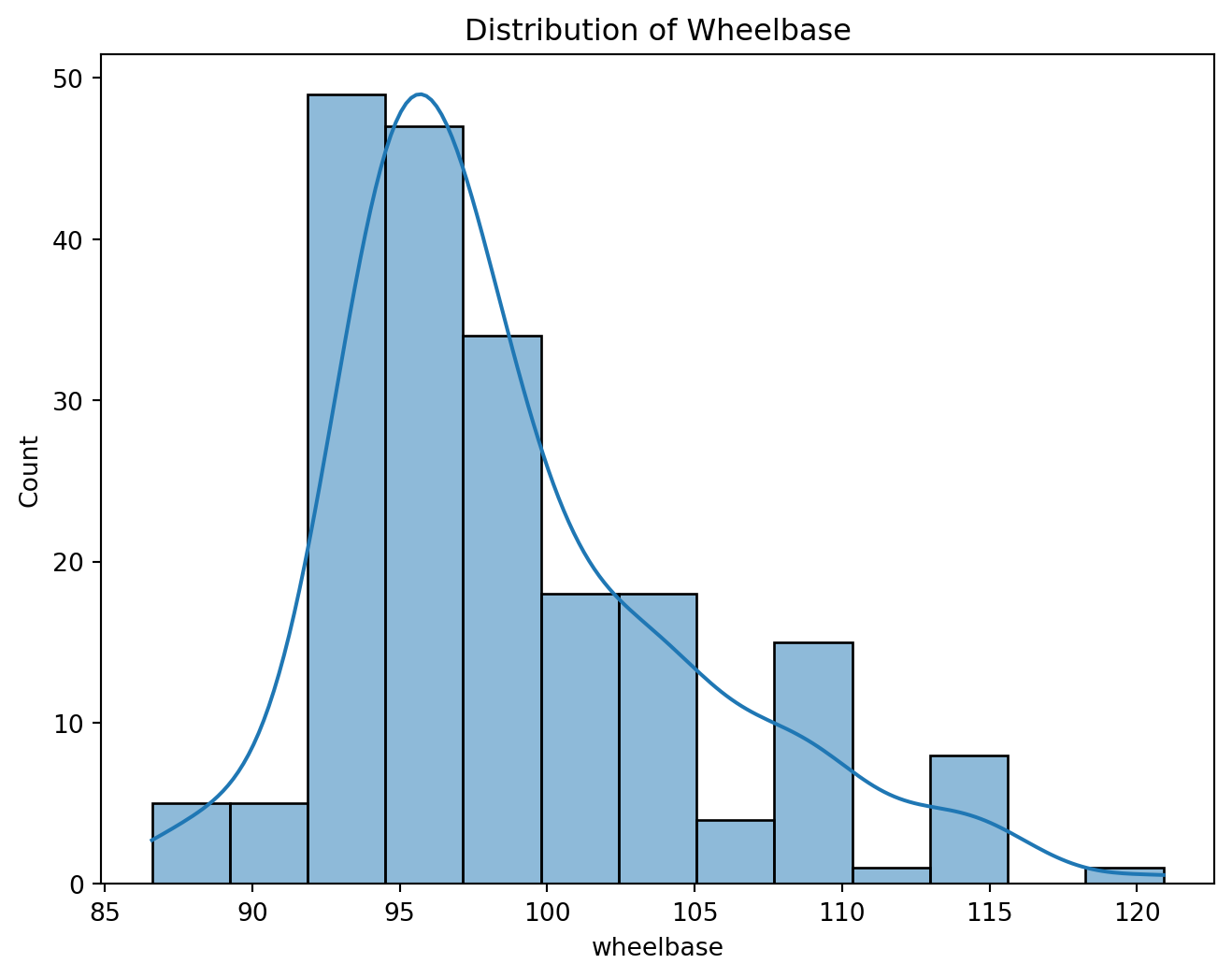

plt.figure(figsize=(8, 6))
sns.histplot(df['carlength'], kde=True)
plt.title('Distribution of Car Length')
plt.show()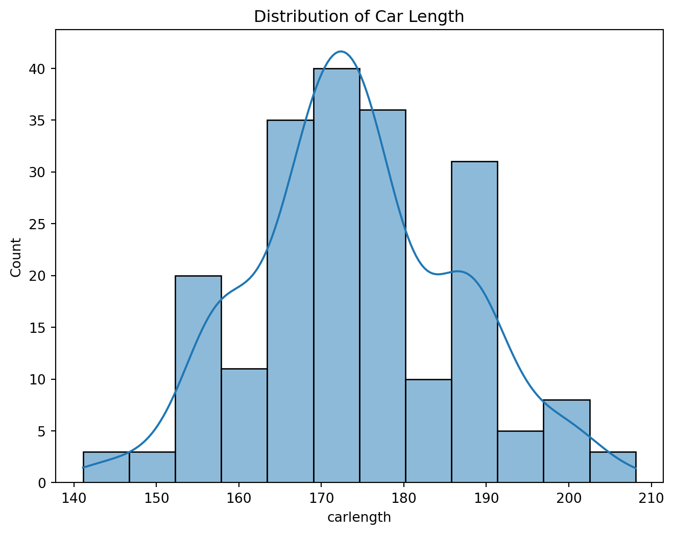

plt.figure(figsize=(8, 6))
sns.histplot(df['carlength'], kde=True)
plt.title('Distribution of Car Length')
plt.show()

plt.figure(figsize=(8, 6))
sns.histplot(df['carheight'], kde=True)
plt.title('Distribution of Car Height')
plt.show()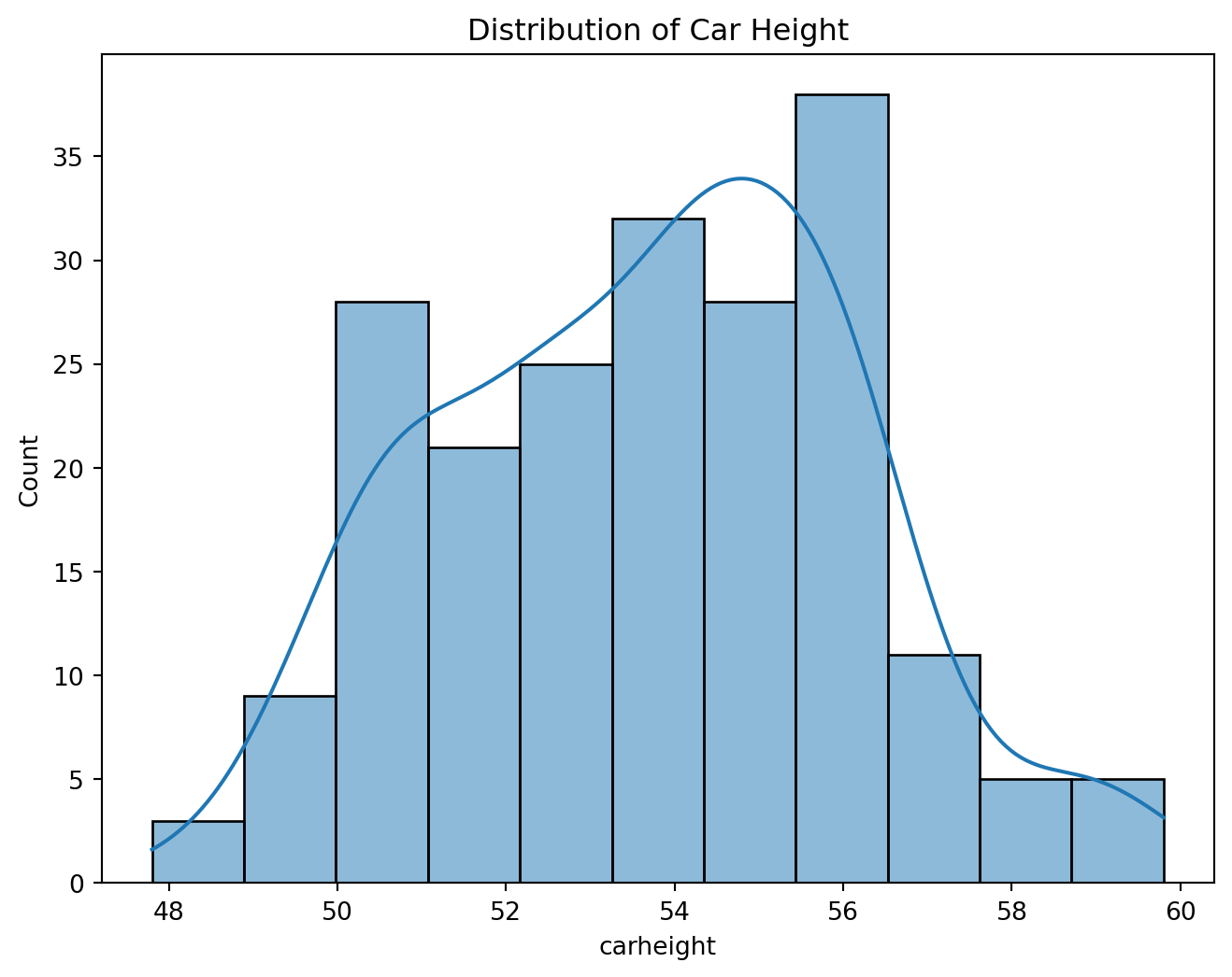

plt.figure(figsize=(8, 6))
sns.histplot(df['curbweight'], kde=True)
plt.title('Distribution of Curb Weight')
plt.show()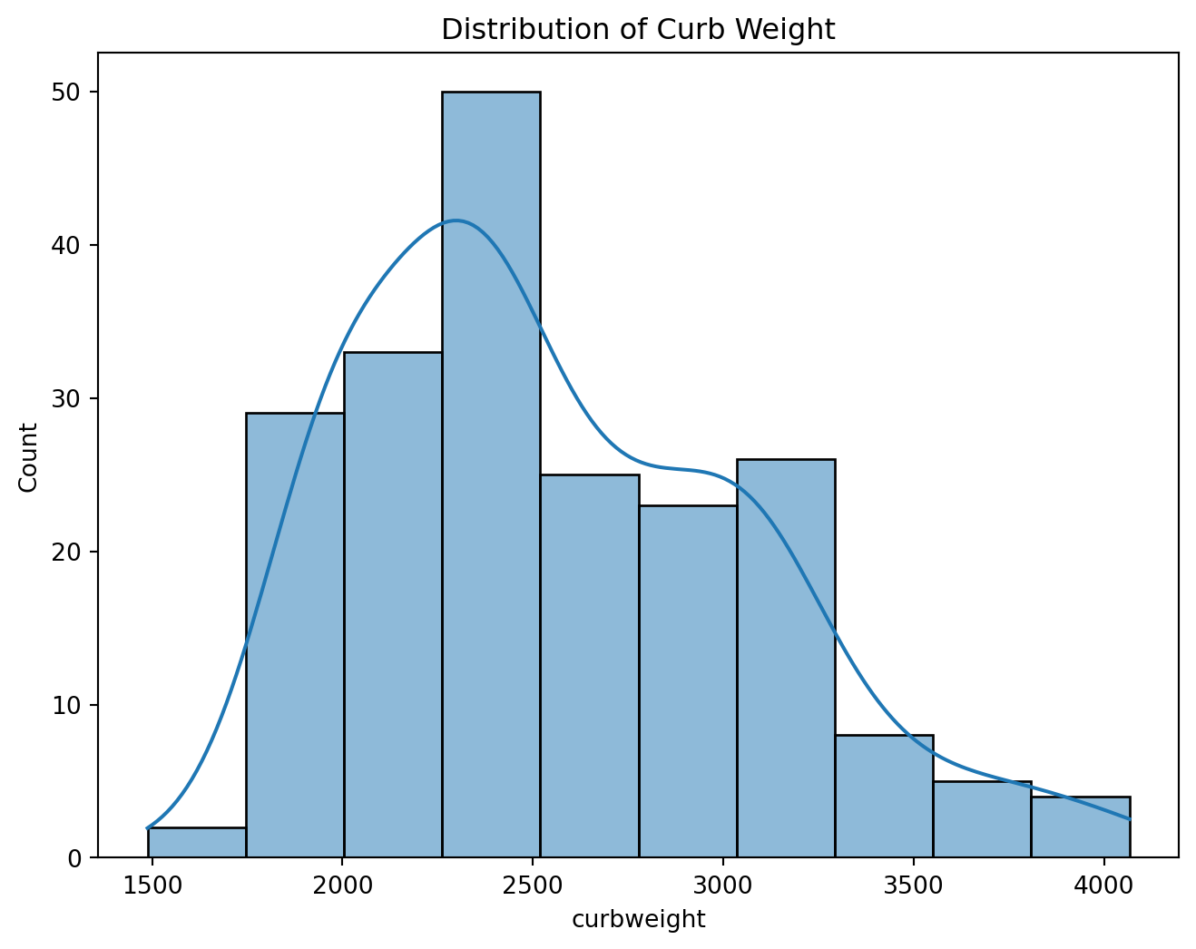

plt.scatter(df['enginesize'], df['price'])
plt.xlabel('Engine Size')
plt.ylabel('Price')
plt.title('Scatter Plot between Engine Size and Price')
plt.show()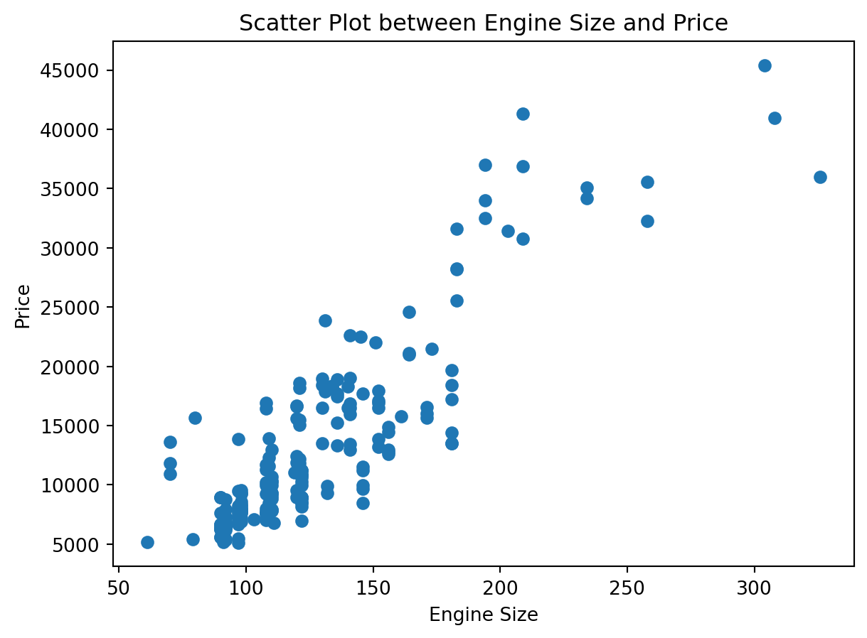

sns.scatterplot(x='horsepower', y='price', data=df)
plt.title('Horsepower vs. Price (Scatter Plot)')
plt.show()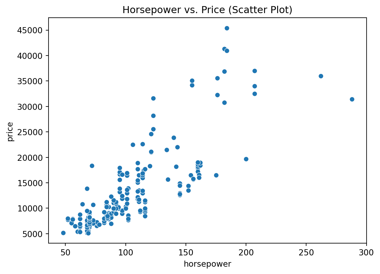

sns.histplot(df['price'], kde=True, color='skyblue')
plt.title('Distribution of Car Prices with KDE')
plt.show()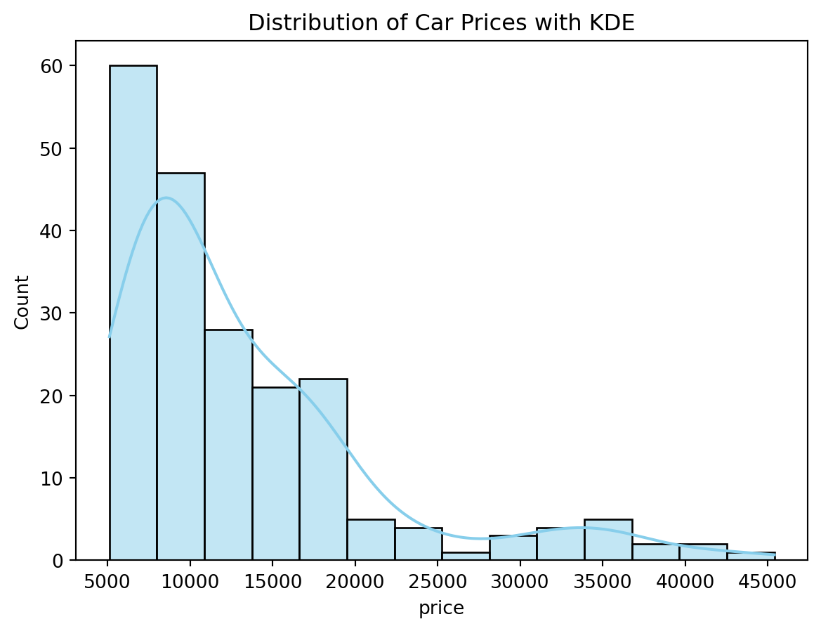

sns.histplot(df['citympg'], kde=True, bins=20, color='skyblue')
plt.title('Distribution of City MPG')
plt.xlabel('City MPG')
plt.show()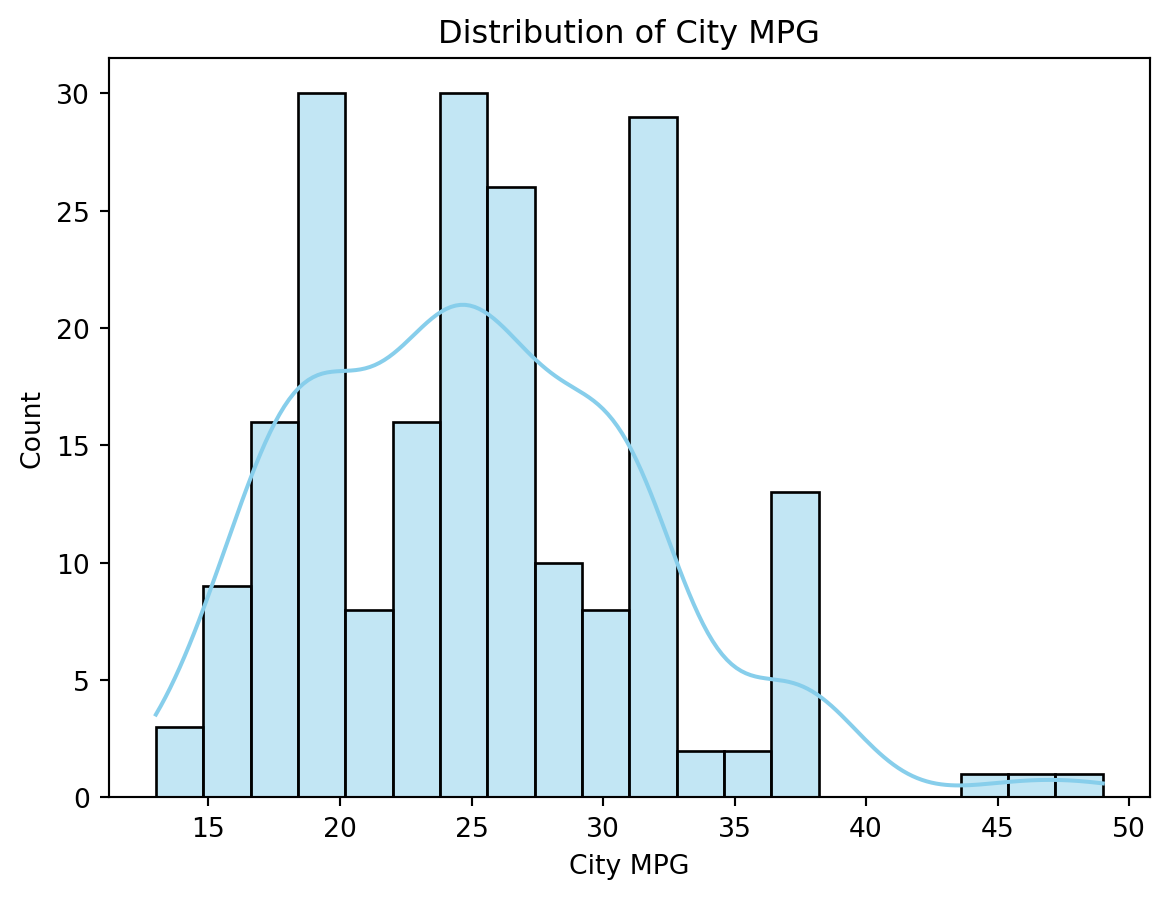

from sklearn.model_selection import train_test_split
X_train,X_test,y_train,y_test=train_test_split(X,y,test_size=0.25,random_state=42)

sns.regplot(x='wheelbase', y='price', data=df, scatter_kws={'s': 20}, line_kws={'color': 'red'})
plt.title('Wheelbase vs. Price')
plt.xlabel('Wheelbase')
plt.ylabel('Price')
plt.show()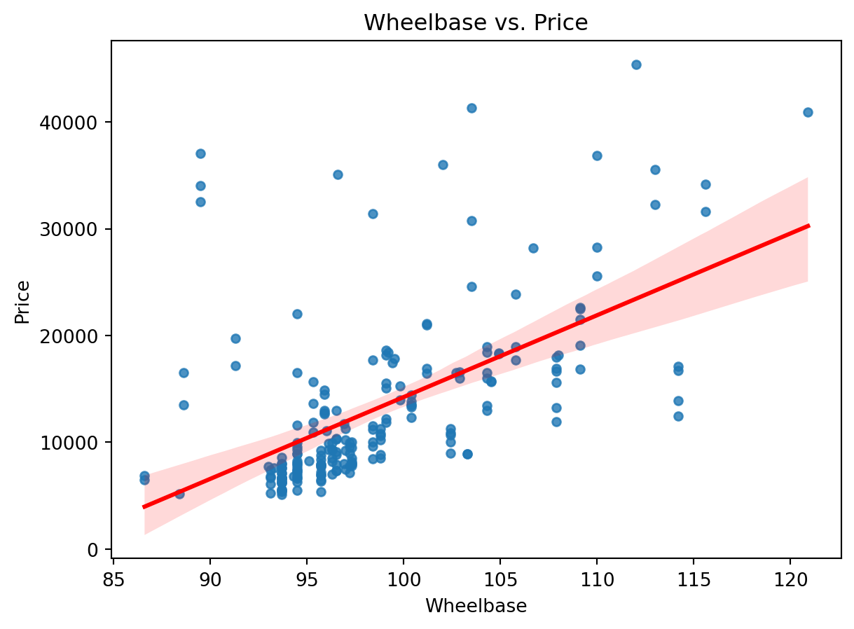

sns.regplot(x='carlength', y='price', data=df, scatter_kws={'s': 20}, line_kws={'color': 'red'})
plt.title('Car Length vs. Price')
plt.xlabel('Car Length')
plt.ylabel('Price')
plt.show()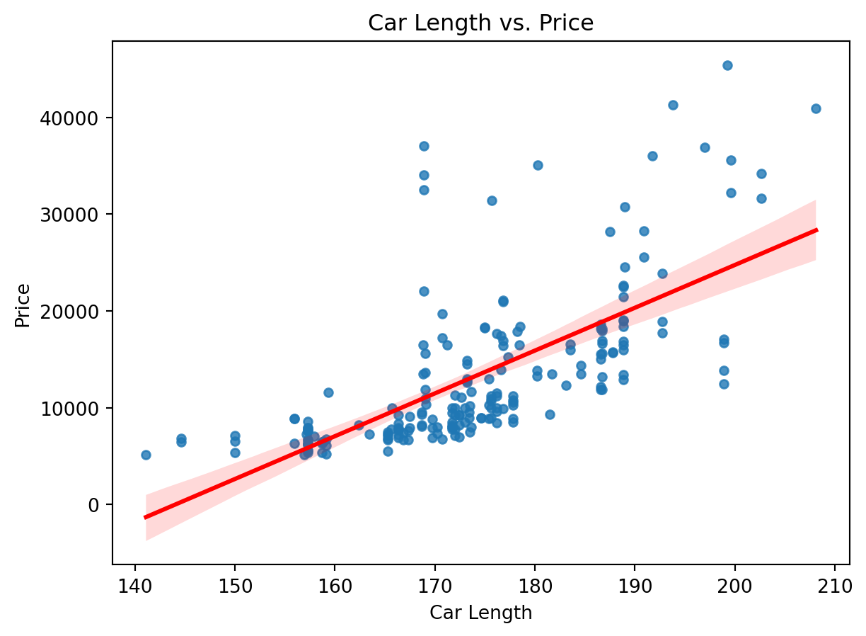

sns.regplot(x='curbweight', y='price', data=df, scatter_kws={'s': 20}, line_kws={'color': 'red'})
plt.title('Curb Weight vs. Price')
plt.xlabel('Curb Weight')
plt.ylabel('Price')
plt.show()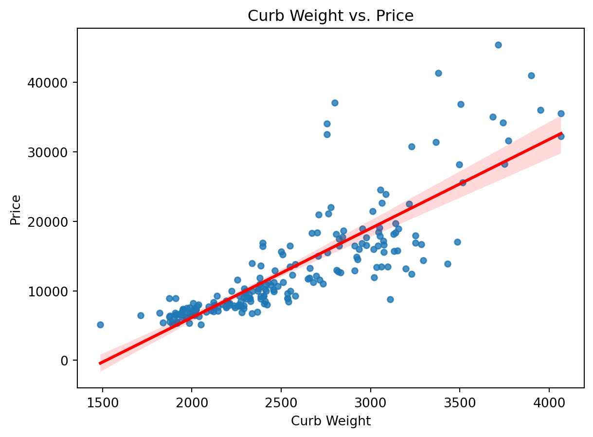

sns.regplot(x='enginesize', y='price', data=df, scatter_kws={'s': 20}, line_kws={'color': 'red'})
plt.title('Engine Size vs. Price')
plt.xlabel('Engine Size')
plt.ylabel('Price')
plt.show()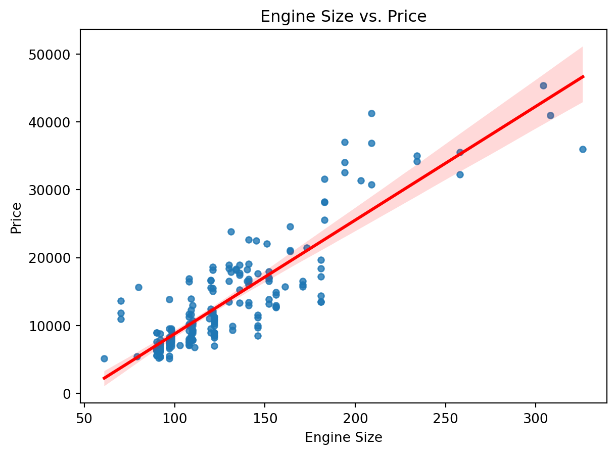

sns.regplot(x='horsepower', y='price', data=df, scatter_kws={'s': 20}, line_kws={'color': 'red'})
plt.title('Horsepower vs. Price')
plt.xlabel('Horsepower')
plt.ylabel('Price')
plt.show()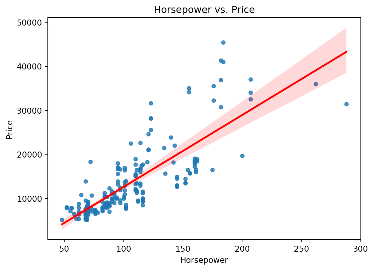

sns.regplot(x='citympg', y='price', data=df, scatter_kws={'s': 20}, line_kws={'color': 'red'})
plt.title('City MPG vs. Price')
plt.xlabel('City MPG')
plt.ylabel('Price')
plt.show()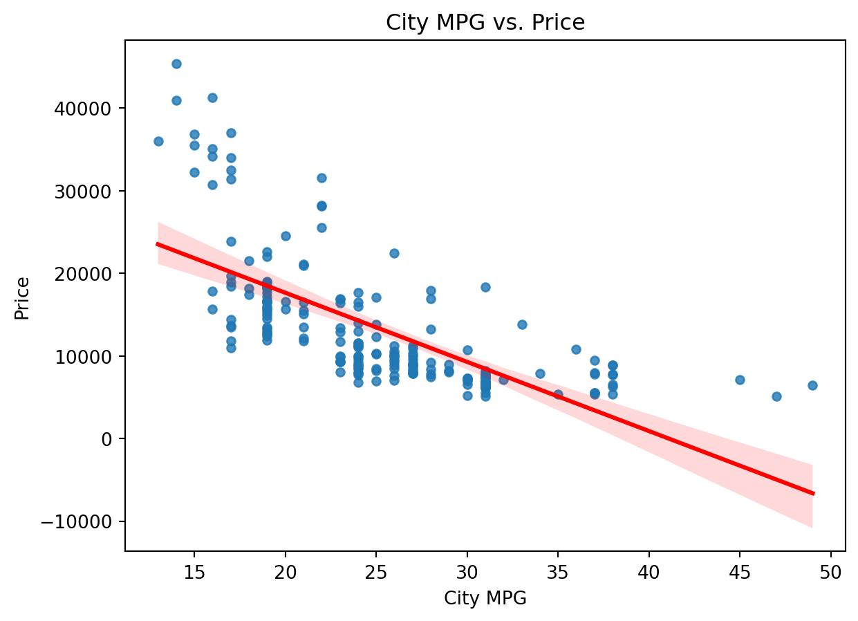

print(X_train.columns)

Index(['wheelbase', 'carlength', 'carwidth', 'carheight', 'curbweight',
       'enginesize', 'boreratio', 'stroke', 'compressionratio', 'horsepower',
       'peakrpm', 'citympg', 'highwaympg'],
      dtype='object')

import pandas as pd
categorical_cols = ['enginesize', 'horsepower', 'peakrpm']
X_train_encoded = pd.get_dummies(X_train, columns=categorical_cols)
X_test_encoded = pd.get_dummies(X_test, columns=categorical_cols)

for column in X_train.columns:
    unique_values = X_train[column].nunique()
    print(f"Column '{column}' has {unique_values} unique values.")

Column 'wheelbase' has 46 unique values.
Column 'carlength' has 63 unique values.
Column 'carwidth' has 41 unique values.
Column 'carheight' has 47 unique values.
Column 'curbweight' has 132 unique values.
Column 'enginesize' has 41 unique values.
Column 'boreratio' has 36 unique values.
Column 'stroke' has 35 unique values.
Column 'compressionratio' has 30 unique values.
Column 'horsepower' has 53 unique values.
Column 'peakrpm' has 23 unique values.
Column 'citympg' has 27 unique values.
Column 'highwaympg' has 28 unique values.

from sklearn.linear_model import LinearRegression
regression=LinearRegression()

for col in categorical_cols:
    print(f"Unique values in '{col}': {X_train[col].unique()}")

Unique values in 'enginesize': [103 122  97 136 146  70 194  92 108 181 140 110 164 151  98 121  91 120
 156  90 141 134 152 119 130  79 109 183 145 258 111 326 161 131 132 209
 234 171  80 203 304]
Unique values in 'horsepower': [ 55  92  69 110 116 101 207  68  82 160 175  73  76 121 143 100  70  95
 112 145 102 114 142 154  90  88  84 162 115  60  97  62 111  52  85 123
 106  86 176  56  78 200 262 156 140 182 155  64 135 288 152 184 161]
Unique values in 'peakrpm': [4800 4200 5200 5500 6000 5900 5000 4500 4250 4400 6600 5800 5400 5600
 4900 4150 5250 5100 4350 4750 4650 5300 5750]

print(X_train.dtypes)

wheelbase           float64
carlength           float64
carwidth            float64
carheight           float64
curbweight            int64
enginesize            int64
boreratio           float64
stroke              float64
compressionratio    float64
horsepower            int64
peakrpm               int64
citympg               int64
highwaympg            int64
dtype: object

X_train_encoded = pd.get_dummies(X_train, columns=categorical_cols)

X_train_encoded = pd.get_dummies(X_train, columns=categorical_cols)
X_test_encoded = pd.get_dummies(X_test, columns=categorical_cols)

non_numeric_cols_train = X_train_encoded.select_dtypes(exclude=['float64', 'int64']).columns
non_numeric_cols_test = X_test_encoded.select_dtypes(exclude=['float64', 'int64']).columns
print("Non-numeric columns in X_train_encoded:", non_numeric_cols_train)
print("Non-numeric columns in X_test_encoded:", non_numeric_cols_test)

Non-numeric columns in X_train_encoded: Index(['enginesize_70', 'enginesize_79', 'enginesize_80', 'enginesize_90',
       'enginesize_91', 'enginesize_92', 'enginesize_97', 'enginesize_98',
       'enginesize_103', 'enginesize_108',
       ...
       'peakrpm_5250', 'peakrpm_5300', 'peakrpm_5400', 'peakrpm_5500',
       'peakrpm_5600', 'peakrpm_5750', 'peakrpm_5800', 'peakrpm_5900',
       'peakrpm_6000', 'peakrpm_6600'],
      dtype='object', length=117)
Non-numeric columns in X_test_encoded: Index(['enginesize_61', 'enginesize_70', 'enginesize_90', 'enginesize_92',
       'enginesize_97', 'enginesize_98', 'enginesize_108', 'enginesize_110',
       'enginesize_120', 'enginesize_121', 'enginesize_122', 'enginesize_131',
       'enginesize_134', 'enginesize_136', 'enginesize_140', 'enginesize_141',
       'enginesize_146', 'enginesize_152', 'enginesize_156', 'enginesize_171',
       'enginesize_173', 'enginesize_181', 'enginesize_183', 'enginesize_209',
       'enginesize_308', 'horsepower_48', 'horsepower_52', 'horsepower_56',
       'horsepower_58', 'horsepower_62', 'horsepower_68', 'horsepower_69',
       'horsepower_70', 'horsepower_72', 'horsepower_73', 'horsepower_82',
       'horsepower_84', 'horsepower_86', 'horsepower_88', 'horsepower_92',
       'horsepower_94', 'horsepower_95', 'horsepower_97', 'horsepower_101',
       'horsepower_102', 'horsepower_110', 'horsepower_111', 'horsepower_114',
       'horsepower_116', 'horsepower_120', 'horsepower_123', 'horsepower_134',
       'horsepower_145', 'horsepower_152', 'horsepower_160', 'horsepower_161',
       'horsepower_182', 'horsepower_184', 'peakrpm_4150', 'peakrpm_4200',
       'peakrpm_4350', 'peakrpm_4400', 'peakrpm_4500', 'peakrpm_4800',
       'peakrpm_5000', 'peakrpm_5100', 'peakrpm_5200', 'peakrpm_5250',
       'peakrpm_5400', 'peakrpm_5500', 'peakrpm_5800', 'peakrpm_6000'],
      dtype='object')

from sklearn.preprocessing import LabelEncoder
label_encoder_train = LabelEncoder()
for col in non_numeric_cols_train:
    X_train_encoded[col] = label_encoder_train.fit_transform(X_train_encoded[col])

label_encoder_test = LabelEncoder()
for col in non_numeric_cols_test:
    X_test_encoded[col] = label_encoder_test.fit_transform(X_test_encoded[col])

for col in non_numeric_cols_train:
    print(f"Unique values in {col}: {X_train_encoded[col].unique()}")

Unique values in enginesize_70: [0 1]
Unique values in enginesize_79: [0 1]
Unique values in enginesize_80: [0 1]
Unique values in enginesize_90: [0 1]
Unique values in enginesize_91: [0 1]
Unique values in enginesize_92: [0 1]
Unique values in enginesize_97: [0 1]
Unique values in enginesize_98: [0 1]
Unique values in enginesize_103: [1 0]
Unique values in enginesize_108: [0 1]
Unique values in enginesize_109: [0 1]
Unique values in enginesize_110: [0 1]
Unique values in enginesize_111: [0 1]
Unique values in enginesize_119: [0 1]
Unique values in enginesize_120: [0 1]
Unique values in enginesize_121: [0 1]
Unique values in enginesize_122: [0 1]
Unique values in enginesize_130: [0 1]
Unique values in enginesize_131: [0 1]
Unique values in enginesize_132: [0 1]
Unique values in enginesize_134: [0 1]
Unique values in enginesize_136: [0 1]
Unique values in enginesize_140: [0 1]
Unique values in enginesize_141: [0 1]
Unique values in enginesize_145: [0 1]
Unique values in enginesize_146: [0 1]
Unique values in enginesize_151: [0 1]
Unique values in enginesize_152: [0 1]
Unique values in enginesize_156: [0 1]
Unique values in enginesize_161: [0 1]
Unique values in enginesize_164: [0 1]
Unique values in enginesize_171: [0 1]
Unique values in enginesize_181: [0 1]
Unique values in enginesize_183: [0 1]
Unique values in enginesize_194: [0 1]
Unique values in enginesize_203: [0 1]
Unique values in enginesize_209: [0 1]
Unique values in enginesize_234: [0 1]
Unique values in enginesize_258: [0 1]
Unique values in enginesize_304: [0 1]
Unique values in enginesize_326: [0 1]
Unique values in horsepower_52: [0 1]
Unique values in horsepower_55: [1 0]
Unique values in horsepower_56: [0 1]
Unique values in horsepower_60: [0 1]
Unique values in horsepower_62: [0 1]
Unique values in horsepower_64: [0 1]
Unique values in horsepower_68: [0 1]
Unique values in horsepower_69: [0 1]
Unique values in horsepower_70: [0 1]
Unique values in horsepower_73: [0 1]
Unique values in horsepower_76: [0 1]
Unique values in horsepower_78: [0 1]
Unique values in horsepower_82: [0 1]
Unique values in horsepower_84: [0 1]
Unique values in horsepower_85: [0 1]
Unique values in horsepower_86: [0 1]
Unique values in horsepower_88: [0 1]
Unique values in horsepower_90: [0 1]
Unique values in horsepower_92: [0 1]
Unique values in horsepower_95: [0 1]
Unique values in horsepower_97: [0 1]
Unique values in horsepower_100: [0 1]
Unique values in horsepower_101: [0 1]
Unique values in horsepower_102: [0 1]
Unique values in horsepower_106: [0 1]
Unique values in horsepower_110: [0 1]
Unique values in horsepower_111: [0 1]
Unique values in horsepower_112: [0 1]
Unique values in horsepower_114: [0 1]
Unique values in horsepower_115: [0 1]
Unique values in horsepower_116: [0 1]
Unique values in horsepower_121: [0 1]
Unique values in horsepower_123: [0 1]
Unique values in horsepower_135: [0 1]
Unique values in horsepower_140: [0 1]
Unique values in horsepower_142: [0 1]
Unique values in horsepower_143: [0 1]
Unique values in horsepower_145: [0 1]
Unique values in horsepower_152: [0 1]
Unique values in horsepower_154: [0 1]
Unique values in horsepower_155: [0 1]
Unique values in horsepower_156: [0 1]
Unique values in horsepower_160: [0 1]
Unique values in horsepower_161: [0 1]
Unique values in horsepower_162: [0 1]
Unique values in horsepower_175: [0 1]
Unique values in horsepower_176: [0 1]
Unique values in horsepower_182: [0 1]
Unique values in horsepower_184: [0 1]
Unique values in horsepower_200: [0 1]
Unique values in horsepower_207: [0 1]
Unique values in horsepower_262: [0 1]
Unique values in horsepower_288: [0 1]
Unique values in peakrpm_4150: [0 1]
Unique values in peakrpm_4200: [0 1]
Unique values in peakrpm_4250: [0 1]
Unique values in peakrpm_4350: [0 1]
Unique values in peakrpm_4400: [0 1]
Unique values in peakrpm_4500: [0 1]
Unique values in peakrpm_4650: [0 1]
Unique values in peakrpm_4750: [0 1]
Unique values in peakrpm_4800: [1 0]
Unique values in peakrpm_4900: [0 1]
Unique values in peakrpm_5000: [0 1]
Unique values in peakrpm_5100: [0 1]
Unique values in peakrpm_5200: [0 1]
Unique values in peakrpm_5250: [0 1]
Unique values in peakrpm_5300: [0 1]
Unique values in peakrpm_5400: [0 1]
Unique values in peakrpm_5500: [0 1]
Unique values in peakrpm_5600: [0 1]
Unique values in peakrpm_5750: [0 1]
Unique values in peakrpm_5800: [0 1]
Unique values in peakrpm_5900: [0 1]
Unique values in peakrpm_6000: [0 1]
Unique values in peakrpm_6600: [0 1]

for col in non_numeric_cols_test:
    print(f"Unique values in {col}: {X_test_encoded[col].unique()}")

Unique values in enginesize_61: [0 1]
Unique values in enginesize_70: [0 1]
Unique values in enginesize_90: [0 1]
Unique values in enginesize_92: [0 1]
Unique values in enginesize_97: [0 1]
Unique values in enginesize_98: [0 1]
Unique values in enginesize_108: [0 1]
Unique values in enginesize_110: [0 1]
Unique values in enginesize_120: [0 1]
Unique values in enginesize_121: [0 1]
Unique values in enginesize_122: [0 1]
Unique values in enginesize_131: [0 1]
Unique values in enginesize_134: [0 1]
Unique values in enginesize_136: [0 1]
Unique values in enginesize_140: [0 1]
Unique values in enginesize_141: [0 1]
Unique values in enginesize_146: [0 1]
Unique values in enginesize_152: [0 1]
Unique values in enginesize_156: [0 1]
Unique values in enginesize_171: [0 1]
Unique values in enginesize_173: [0 1]
Unique values in enginesize_181: [0 1]
Unique values in enginesize_183: [0 1]
Unique values in enginesize_209: [1 0]
Unique values in enginesize_308: [0 1]
Unique values in horsepower_48: [0 1]
Unique values in horsepower_52: [0 1]
Unique values in horsepower_56: [0 1]
Unique values in horsepower_58: [0 1]
Unique values in horsepower_62: [0 1]
Unique values in horsepower_68: [0 1]
Unique values in horsepower_69: [0 1]
Unique values in horsepower_70: [0 1]
Unique values in horsepower_72: [0 1]
Unique values in horsepower_73: [0 1]
Unique values in horsepower_82: [0 1]
Unique values in horsepower_84: [0 1]
Unique values in horsepower_86: [0 1]
Unique values in horsepower_88: [0 1]
Unique values in horsepower_92: [0 1]
Unique values in horsepower_94: [0 1]
Unique values in horsepower_95: [0 1]
Unique values in horsepower_97: [0 1]
Unique values in horsepower_101: [0 1]
Unique values in horsepower_102: [0 1]
Unique values in horsepower_110: [0 1]
Unique values in horsepower_111: [0 1]
Unique values in horsepower_114: [0 1]
Unique values in horsepower_116: [0 1]
Unique values in horsepower_120: [0 1]
Unique values in horsepower_123: [0 1]
Unique values in horsepower_134: [0 1]
Unique values in horsepower_145: [0 1]
Unique values in horsepower_152: [0 1]
Unique values in horsepower_160: [0 1]
Unique values in horsepower_161: [0 1]
Unique values in horsepower_182: [1 0]
Unique values in horsepower_184: [0 1]
Unique values in peakrpm_4150: [0 1]
Unique values in peakrpm_4200: [0 1]
Unique values in peakrpm_4350: [0 1]
Unique values in peakrpm_4400: [0 1]
Unique values in peakrpm_4500: [0 1]
Unique values in peakrpm_4800: [0 1]
Unique values in peakrpm_5000: [0 1]
Unique values in peakrpm_5100: [0 1]
Unique values in peakrpm_5200: [0 1]
Unique values in peakrpm_5250: [0 1]
Unique values in peakrpm_5400: [1 0]
Unique values in peakrpm_5500: [0 1]
Unique values in peakrpm_5800: [0 1]
Unique values in peakrpm_6000: [0 1]

from sklearn.preprocessing import LabelEncoder, OneHotEncoder
label_encoder = LabelEncoder()

for col in categorical_cols:
    X_train[col] = label_encoder.fit_transform(X_train[col])

onehot_encoder = OneHotEncoder(drop='first', sparse=False)

X_train_encoded = pd.get_dummies(X_train, columns=categorical_cols, drop_first=True)
X_test_encoded = pd.get_dummies(X_test, columns=categorical_cols, drop_first=True)

X_train_encoded, X_test_encoded = X_train_encoded.align(X_test_encoded, join='outer', axis=1, fill_value=0)

regression.fit(X_train_encoded, y_train)

LinearRegression()

In a Jupyter environment, please rerun this cell to show the HTML representation or trust the notebook.
On GitHub, the HTML representation is unable to render, please try loading this page with nbviewer.org.

from sklearn.model_selection import cross_val_score
validation_score=cross_val_score(regression,X_train,y_train,scoring='neg_mean_squared_error',
                             cv=3)

np.mean(validation_score)

-17619779.964257453

y_pred = regression.predict(X_test_encoded)
y_pred

array([ 17663.40920114,   2843.49700864,   -681.0197125 ,  20031.97260338,
        23256.22526061,  -2078.06829731,  11404.65164046,   8303.95517846,
        34989.85861164,  -1974.8074486 ,    672.29083674,   7942.30385746,
        26485.26793673,  -1324.44214526,  31219.07729321,   3691.87875078,
        -5254.23835884,   -389.77808369,   1982.84977136,  34302.79230783,
         4217.87918551,  15554.97366416,  -1635.32099728, -14421.58919858,
        -3894.410904  ,  18993.50244592,  10010.82968533,  28157.3938917 ,
        -2754.23702629,  27383.42715415,  21693.84435239,  -4089.13068506,
         3223.28302425,  32429.56926617,  -6839.56578167,  21720.24707413,
        34377.53936716,   9197.98033432,    136.89843489,    723.50606337,
        32982.56263849,  11575.29609297,  49483.4797775 ,   3077.1128973 ,
        -2818.66172925,  -8107.23857484,  -4089.13068506,  32626.79986009,
        25793.48112021,  -1219.70262027,   -172.88303499,   8578.30732609])

from sklearn.metrics import mean_absolute_error,mean_squared_error
mse=mean_squared_error(y_test,y_pred)
mae=mean_absolute_error(y_test,y_pred)
rmse=np.sqrt(mse)
print(mse)
print(mae)
print(rmse)

177304634.11961922
11133.618219594775
13315.57862503989

from sklearn.metrics import r2_score
score=r2_score(y_test,y_pred)
print(score)
print(1 - (1-score)*(len(y_test)-1)/(len(y_test)-X_test.shape[1]-1))

-1.6205416455966546
-2.51704273487972

plt.scatter(y_test,y_pred)

<matplotlib.collections.PathCollection at 0x276300a7c50>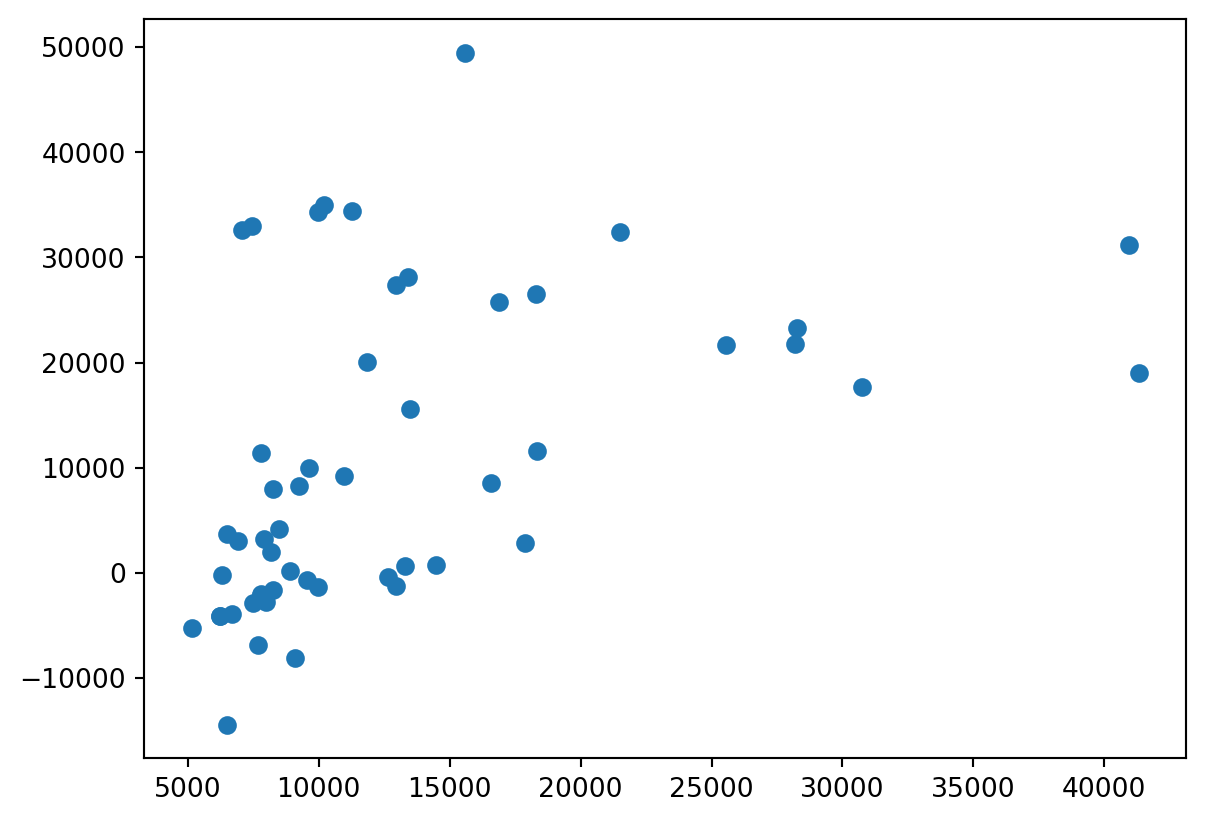

residuals=y_test-y_pred
print(residuals)

15     13096.590799
9      15015.669991
100    10230.019713
132    -8181.972603
68      4991.774739
95      9877.068297
159    -3616.651640
162      954.044822
147   -24791.858612
182     9749.807449
191    12622.709163
164      295.696143
65     -8205.267937
175    11312.442145
73      9740.922707
152     2796.121249
18     10405.238359
82     13018.778084
86      6206.150229
143   -24342.792308
60      4277.120814
101    -2055.973664
98      9884.320997
30     20900.589199
25     10586.410904
16     22321.497554
168     -371.829685
195   -14742.393892
97     10753.237026
194   -14443.427154
67      3858.155648
120    10318.130685
154     4674.716976
202   -10944.569266
79     14528.565782
69      6455.752926
145   -23118.539367
55      1747.019666
45      8779.601565
84     13765.493937
146   -25519.562638
66      6768.703907
111   -33903.479777
153     3840.887103
96     10317.661729
38     17202.238575
24     10318.130685
139   -25573.799860
112    -8893.481120
29     14183.702620
19      6467.883035
178     7979.692674
Name: price, dtype: float64

sns.displot(residuals,kind='kde')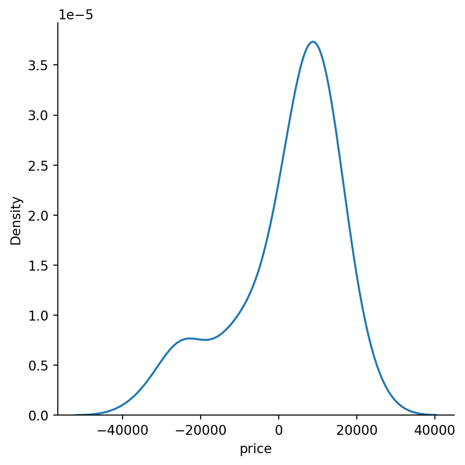

plt.scatter(y_pred,residuals)

<matplotlib.collections.PathCollection at 0x27635afdcd0>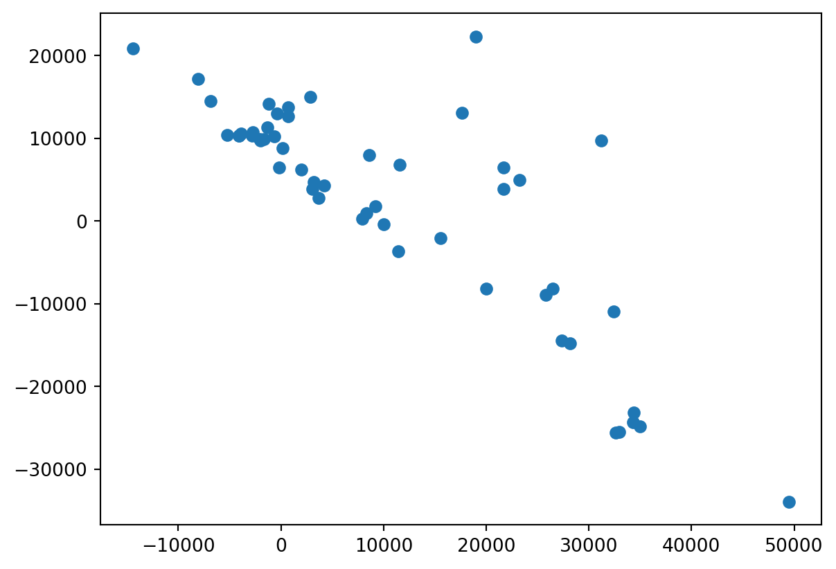

sns.histplot(y_pred, kde=True, color='skyblue')
plt.title('Distribution of Predicted Prices')
plt.xlabel('Predicted Prices')
plt.show()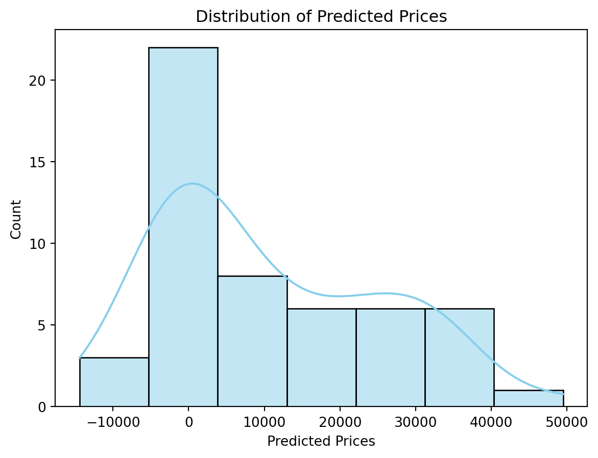

3.b)Non-Linear Regression

What is a Non-Linear Regression?

One kind of polynomial regression is non-linear regression. A non-linear relationship between the dependent and independent variables can be modeled using this technique. When the data exhibits a curved trend and non-linear regression yields more accurate results than linear regression, it is used instead of linear regression. This is because the assumption behind linear regression is that the data is linear.

How does a Non-Linear Regression work?

When we pay close attention, we will see that non-linear regression is the next step up from linear regression. All that needs to be done is add the dependent features' higher-order terms to the feature space. Though not precisely, feature engineering is another name for this at times.

Applications of Non-Linear Regression

that non-linear regression techniques are superior to linear regression techniques because most real-world data is non-linear. Non-linear regression methods aid in the creation of a solid model whose forecasts are trustworthy and consistent with the historical trend observed in the data. Non-Linear Regression techniques successfully completed tasks related to logistic pricing model, financial forecasting, and exponential growth or decay of a population.

from sklearn.ensemble import GradientBoostingRegressor
import numpy as np
import pandas as pd
from sklearn.model_selection import train_test_split
from sklearn.metrics import mean_squared_error
from sklearn.metrics import mean_absolute_error
from sklearn.metrics import r2_score
from sklearn.datasets import load_iris
from sklearn.model_selection import train_test_split, GridSearchCV
import warnings
import seaborn as sns
import matplotlib.pyplot as plt
warnings.filterwarnings('ignore')

df = pd.read_csv('miami-housing.csv')
df.head()

	LATITUDE	LONGITUDE	PARCELNO	SALE_PRC	LND_SQFOOT	TOT_LVG_AREA	SPEC_FEAT_VAL	RAIL_DIST	OCEAN_DIST	WATER_DIST	CNTR_DIST	SUBCNTR_DI	HWY_DIST	age	month_sold	structure_quality
0	25.891031	-80.160561	622280070620	440000.0	9375	1753	0	2815.9	12811.4	347.6	42815.3	37742.2	15954.9	67	8	4
1	25.891324	-80.153968	622280100460	349000.0	9375	1715	0	4359.1	10648.4	337.8	43504.9	37340.5	18125.0	63	9	4
2	25.891334	-80.153740	622280100470	800000.0	9375	2276	49206	4412.9	10574.1	297.1	43530.4	37328.7	18200.5	61	2	4
3	25.891765	-80.152657	622280100530	988000.0	12450	2058	10033	4585.0	10156.5	0.0	43797.5	37423.2	18514.4	63	9	4
4	25.891825	-80.154639	622280100200	755000.0	12800	1684	16681	4063.4	10836.8	326.6	43599.7	37550.8	17903.4	42	7	4

df.columns

Index(['LATITUDE', 'LONGITUDE', 'PARCELNO', 'SALE_PRC', 'LND_SQFOOT',
       'TOT_LVG_AREA', 'SPEC_FEAT_VAL', 'RAIL_DIST', 'OCEAN_DIST',
       'WATER_DIST', 'CNTR_DIST', 'SUBCNTR_DI', 'HWY_DIST', 'age',
       'avno60plus', 'month_sold', 'structure_quality'],
      dtype='object')

df.info()

<class 'pandas.core.frame.DataFrame'>
RangeIndex: 13932 entries, 0 to 13931
Data columns (total 17 columns):
 #   Column             Non-Null Count  Dtype  
---  ------             --------------  -----  
 0   LATITUDE           13932 non-null  float64
 1   LONGITUDE          13932 non-null  float64
 2   PARCELNO           13932 non-null  int64  
 3   SALE_PRC           13932 non-null  float64
 4   LND_SQFOOT         13932 non-null  int64  
 5   TOT_LVG_AREA       13932 non-null  int64  
 6   SPEC_FEAT_VAL      13932 non-null  int64  
 7   RAIL_DIST          13932 non-null  float64
 8   OCEAN_DIST         13932 non-null  float64
 9   WATER_DIST         13932 non-null  float64
 10  CNTR_DIST          13932 non-null  float64
 11  SUBCNTR_DI         13932 non-null  float64
 12  HWY_DIST           13932 non-null  float64
 13  age                13932 non-null  int64  
 14  avno60plus         13932 non-null  int64  
 15  month_sold         13932 non-null  int64  
 16  structure_quality  13932 non-null  int64  
dtypes: float64(9), int64(8)
memory usage: 1.8 MB

df.describe()

	LATITUDE	LONGITUDE	PARCELNO	SALE_PRC	LND_SQFOOT	TOT_LVG_AREA	SPEC_FEAT_VAL	RAIL_DIST	OCEAN_DIST	WATER_DIST	CNTR_DIST	SUBCNTR_DI	HWY_DIST	age	avno60plus	month_sold	structure_quality
count	13932.000000	13932.000000	1.393200e+04	1.393200e+04	13932.000000	13932.000000	13932.000000	13932.000000	13932.000000	13932.000000	13932.000000	13932.000000	13932.000000	13932.000000	13932.000000	13932.000000	13932.000000
mean	25.728811	-80.327475	2.356496e+12	3.999419e+05	8620.879917	2058.044574	9562.493468	8348.548715	31690.993798	11960.285235	68490.327132	41115.047265	7723.770693	30.669251	0.014930	6.655828	3.513997
std	0.140633	0.089199	1.199290e+12	3.172147e+05	6070.088742	813.538535	13890.967782	6178.027333	17595.079468	11932.992369	32008.474808	22161.825935	6068.936108	21.153068	0.121276	3.301523	1.097444
min	25.434333	-80.542172	1.020008e+11	7.200000e+04	1248.000000	854.000000	0.000000	10.500000	236.100000	0.000000	3825.600000	1462.800000	90.200000	0.000000	0.000000	1.000000	1.000000
25%	25.620056	-80.403278	1.079160e+12	2.350000e+05	5400.000000	1470.000000	810.000000	3299.450000	18079.350000	2675.850000	42823.100000	23996.250000	2998.125000	14.000000	0.000000	4.000000	2.000000
50%	25.731810	-80.338911	3.040300e+12	3.100000e+05	7500.000000	1877.500000	2765.500000	7106.300000	28541.750000	6922.600000	65852.400000	41109.900000	6159.750000	26.000000	0.000000	7.000000	4.000000
75%	25.852269	-80.258019	3.060170e+12	4.280000e+05	9126.250000	2471.000000	12352.250000	12102.600000	44310.650000	19200.000000	89358.325000	53949.375000	10854.200000	46.000000	0.000000	9.000000	4.000000
max	25.974382	-80.119746	3.660170e+12	2.650000e+06	57064.000000	6287.000000	175020.000000	29621.500000	75744.900000	50399.800000	159976.500000	110553.800000	48167.300000	96.000000	1.000000	12.000000	5.000000

df.shape

(13932, 17)

df.isnull()

	LATITUDE	LONGITUDE	PARCELNO	SALE_PRC	LND_SQFOOT	TOT_LVG_AREA	SPEC_FEAT_VAL	RAIL_DIST	OCEAN_DIST	WATER_DIST	CNTR_DIST	SUBCNTR_DI	HWY_DIST	age	avno60plus	month_sold	structure_quality
0	False	False	False	False	False	False	False	False	False	False	False	False	False	False	False	False	False
1	False	False	False	False	False	False	False	False	False	False	False	False	False	False	False	False	False
2	False	False	False	False	False	False	False	False	False	False	False	False	False	False	False	False	False
3	False	False	False	False	False	False	False	False	False	False	False	False	False	False	False	False	False
4	False	False	False	False	False	False	False	False	False	False	False	False	False	False	False	False	False
...	...	...	...	...	...	...	...	...	...	...	...	...	...	...	...	...	...
13927	False	False	False	False	False	False	False	False	False	False	False	False	False	False	False	False	False
13928	False	False	False	False	False	False	False	False	False	False	False	False	False	False	False	False	False
13929	False	False	False	False	False	False	False	False	False	False	False	False	False	False	False	False	False
13930	False	False	False	False	False	False	False	False	False	False	False	False	False	False	False	False	False
13931	False	False	False	False	False	False	False	False	False	False	False	False	False	False	False	False	False

13932 rows × 17 columns

df.dropna(inplace =True)
df.isnull().sum()

LATITUDE             0
LONGITUDE            0
PARCELNO             0
SALE_PRC             0
LND_SQFOOT           0
TOT_LVG_AREA         0
SPEC_FEAT_VAL        0
RAIL_DIST            0
OCEAN_DIST           0
WATER_DIST           0
CNTR_DIST            0
SUBCNTR_DI           0
HWY_DIST             0
age                  0
avno60plus           0
month_sold           0
structure_quality    0
dtype: int64

df.duplicated().any()

False

df.corr()

	LATITUDE	LONGITUDE	PARCELNO	SALE_PRC	LND_SQFOOT	TOT_LVG_AREA	SPEC_FEAT_VAL	RAIL_DIST	OCEAN_DIST	WATER_DIST	CNTR_DIST	SUBCNTR_DI	HWY_DIST	age	avno60plus	month_sold	structure_quality
LATITUDE	1.000000	0.721232	-0.165487	0.047701	-0.077481	-0.193972	-0.007634	-0.172382	0.242735	-0.423396	-0.717348	-0.195823	-0.113443	0.416967	0.081366	-0.023634	0.391989
LONGITUDE	0.721232	1.000000	-0.432816	0.195274	0.018242	-0.181007	-0.009372	-0.303155	-0.457477	-0.764256	-0.791968	-0.380220	-0.216406	0.488757	0.059416	-0.010859	0.132893
PARCELNO	-0.165487	-0.432816	1.000000	-0.204068	0.071381	0.102439	0.055152	0.223387	0.289232	0.295951	0.419933	0.243888	0.018247	-0.270718	-0.160925	0.011129	0.044652
SALE_PRC	0.047701	0.195274	-0.204068	1.000000	0.363077	0.667301	0.497500	-0.077009	-0.274675	-0.127938	-0.271425	-0.370078	0.231877	-0.123408	-0.027026	0.000325	0.383995
LND_SQFOOT	-0.077481	0.018242	0.071381	0.363077	1.000000	0.437472	0.390707	-0.083901	-0.161579	-0.055093	-0.023181	-0.159094	0.130488	0.101244	-0.005899	0.005926	-0.006686
TOT_LVG_AREA	-0.193972	-0.181007	0.102439	0.667301	0.437472	1.000000	0.506064	0.075486	-0.050141	0.148343	0.136526	-0.044882	0.229497	-0.340606	-0.056545	0.002517	0.173422
SPEC_FEAT_VAL	-0.007634	-0.009372	0.055152	0.497500	0.390707	0.506064	1.000000	-0.021965	-0.055155	0.013923	-0.048817	-0.151916	0.153770	-0.098780	-0.008879	-0.014012	0.188030
RAIL_DIST	-0.172382	-0.303155	0.223387	-0.077009	-0.083901	0.075486	-0.021965	1.000000	0.258966	0.162313	0.444494	0.485468	-0.092495	-0.234515	-0.116955	0.010560	-0.074075
OCEAN_DIST	0.242735	-0.457477	0.289232	-0.274675	-0.161579	-0.050141	-0.055155	0.258966	1.000000	0.490764	0.245396	0.425869	0.093500	-0.159409	0.035215	-0.012723	0.209497
WATER_DIST	-0.423396	-0.764256	0.295951	-0.127938	-0.055093	0.148343	0.013923	0.162313	0.490764	1.000000	0.526952	0.195280	0.400233	-0.330578	-0.096339	0.010556	-0.034343
CNTR_DIST	-0.717348	-0.791968	0.419933	-0.271425	-0.023181	0.136526	-0.048817	0.444494	0.245396	0.526952	1.000000	0.766387	0.076484	-0.548287	-0.130857	0.023096	-0.330588
SUBCNTR_DI	-0.195823	-0.380220	0.243888	-0.370078	-0.159094	-0.044882	-0.151916	0.485468	0.425869	0.195280	0.766387	1.000000	-0.093982	-0.385278	-0.073202	0.016334	-0.248656
HWY_DIST	-0.113443	-0.216406	0.018247	0.231877	0.130488	0.229497	0.153770	-0.092495	0.093500	0.400233	0.076484	-0.093982	1.000000	-0.120505	-0.019788	-0.004547	0.193529
age	0.416967	0.488757	-0.270718	-0.123408	0.101244	-0.340606	-0.098780	-0.234515	-0.159409	-0.330578	-0.548287	-0.385278	-0.120505	1.000000	0.110325	-0.038904	0.009253
avno60plus	0.081366	0.059416	-0.160925	-0.027026	-0.005899	-0.056545	-0.008879	-0.116955	0.035215	-0.096339	-0.130857	-0.073202	-0.019788	0.110325	1.000000	-0.020870	0.096050
month_sold	-0.023634	-0.010859	0.011129	0.000325	0.005926	0.002517	-0.014012	0.010560	-0.012723	0.010556	0.023096	0.016334	-0.004547	-0.038904	-0.020870	1.000000	-0.011023
structure_quality	0.391989	0.132893	0.044652	0.383995	-0.006686	0.173422	0.188030	-0.074075	0.209497	-0.034343	-0.330588	-0.248656	0.193529	0.009253	0.096050	-0.011023	1.000000

df.drop(['LONGITUDE', 'WATER_DIST'], axis=1,inplace=True)

low_corr_features = ['PARCELNO', 'age', 'avno60plus', 'month_sold']
df.drop(low_corr_features, axis=1,inplace=True)

df.corr()

	LATITUDE	SALE_PRC	LND_SQFOOT	TOT_LVG_AREA	SPEC_FEAT_VAL	RAIL_DIST	OCEAN_DIST	CNTR_DIST	SUBCNTR_DI	HWY_DIST	structure_quality
LATITUDE	1.000000	0.047701	-0.077481	-0.193972	-0.007634	-0.172382	0.242735	-0.717348	-0.195823	-0.113443	0.391989
SALE_PRC	0.047701	1.000000	0.363077	0.667301	0.497500	-0.077009	-0.274675	-0.271425	-0.370078	0.231877	0.383995
LND_SQFOOT	-0.077481	0.363077	1.000000	0.437472	0.390707	-0.083901	-0.161579	-0.023181	-0.159094	0.130488	-0.006686
TOT_LVG_AREA	-0.193972	0.667301	0.437472	1.000000	0.506064	0.075486	-0.050141	0.136526	-0.044882	0.229497	0.173422
SPEC_FEAT_VAL	-0.007634	0.497500	0.390707	0.506064	1.000000	-0.021965	-0.055155	-0.048817	-0.151916	0.153770	0.188030
RAIL_DIST	-0.172382	-0.077009	-0.083901	0.075486	-0.021965	1.000000	0.258966	0.444494	0.485468	-0.092495	-0.074075
OCEAN_DIST	0.242735	-0.274675	-0.161579	-0.050141	-0.055155	0.258966	1.000000	0.245396	0.425869	0.093500	0.209497
CNTR_DIST	-0.717348	-0.271425	-0.023181	0.136526	-0.048817	0.444494	0.245396	1.000000	0.766387	0.076484	-0.330588
SUBCNTR_DI	-0.195823	-0.370078	-0.159094	-0.044882	-0.151916	0.485468	0.425869	0.766387	1.000000	-0.093982	-0.248656
HWY_DIST	-0.113443	0.231877	0.130488	0.229497	0.153770	-0.092495	0.093500	0.076484	-0.093982	1.000000	0.193529
structure_quality	0.391989	0.383995	-0.006686	0.173422	0.188030	-0.074075	0.209497	-0.330588	-0.248656	0.193529	1.000000

plt.figure(figsize=(8, 6))
sns.histplot(df['CNTR_DIST'], bins=30, kde=True)
plt.title('Distribution of CNTR_DIST')
plt.show()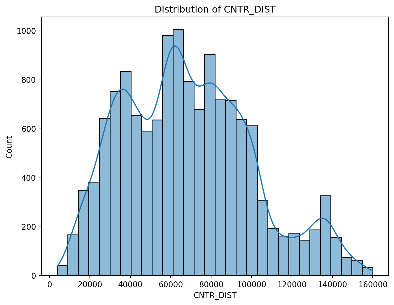

plt.figure(figsize=(8, 6))
sns.regplot(x='OCEAN_DIST', y='SALE_PRC', data=df)
plt.title('Regression plot of OCEAN_DIST vs. SALE_PRC')
plt.show()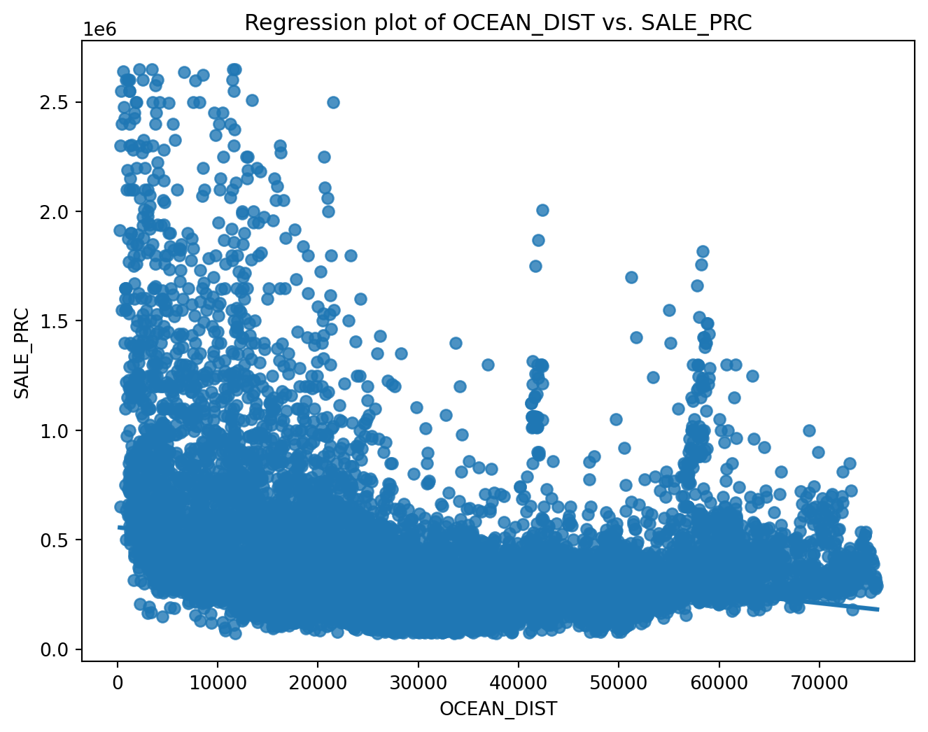

plt.figure(figsize=(8, 6))
sns.scatterplot(x='LND_SQFOOT', y='SALE_PRC', data=df)
plt.title('Scatter plot of LND_SQFOOT vs. SALE_PRC')
plt.show()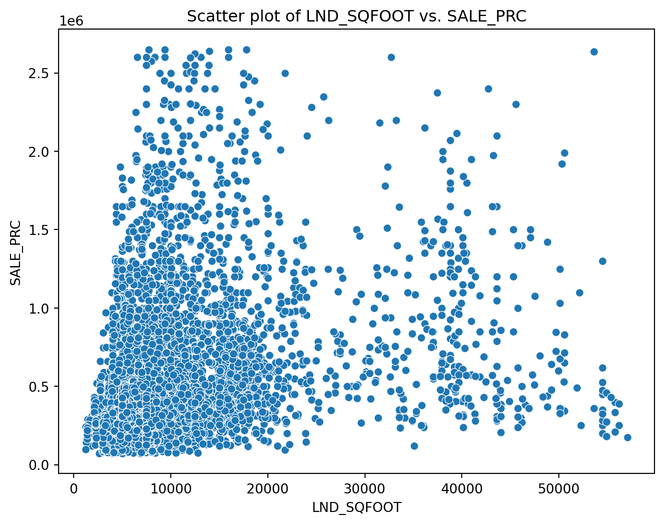

plt.figure(figsize=(8, 6))
sns.histplot(df['SALE_PRC'], bins=30, kde=True)
plt.title('Distribution of SALE_PRC')
plt.show()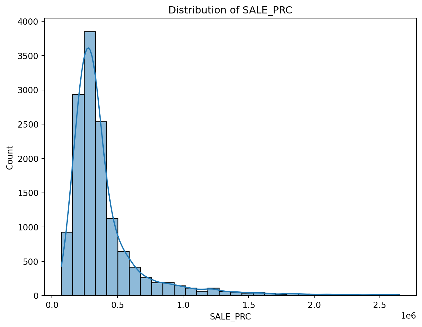

sns.set(style="darkgrid")
color_palette = "viridis"
sns.relplot(x='CNTR_DIST', y='SALE_PRC', sizes=(1, 100), hue='TOT_LVG_AREA', palette=color_palette, size='SALE_PRC', data=df)
plt.xlabel('Distance to Miami Central Business')
plt.ylabel('Sale Price')
plt.ticklabel_format(style='plain', axis='y')
plt.xticks(fontsize=8)
plt.show()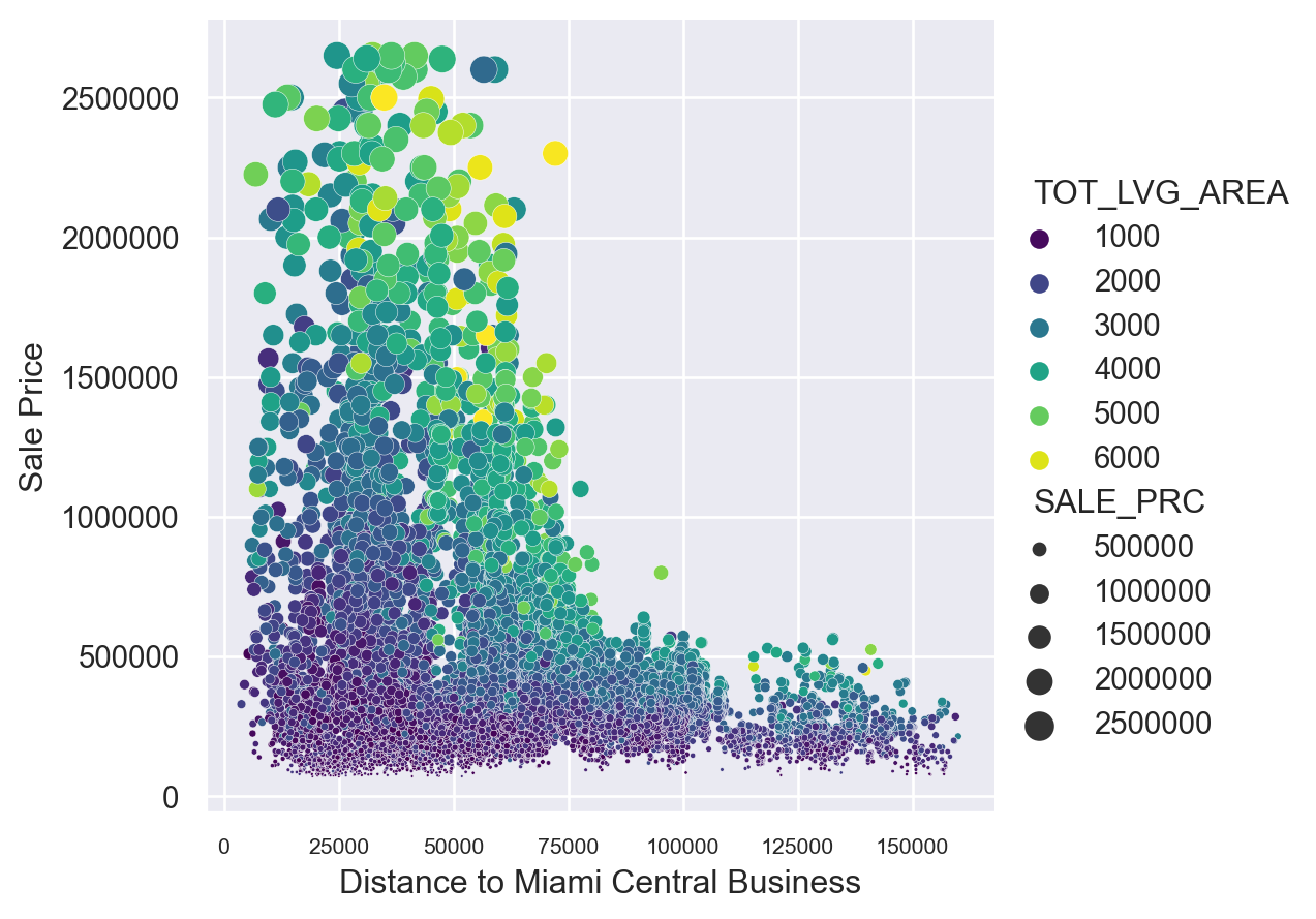

sns.scatterplot(x='HWY_DIST', y='SALE_PRC', data=df)
plt.title('Scatter plot of HWY_DIST vs. SALE_PRC')
plt.show()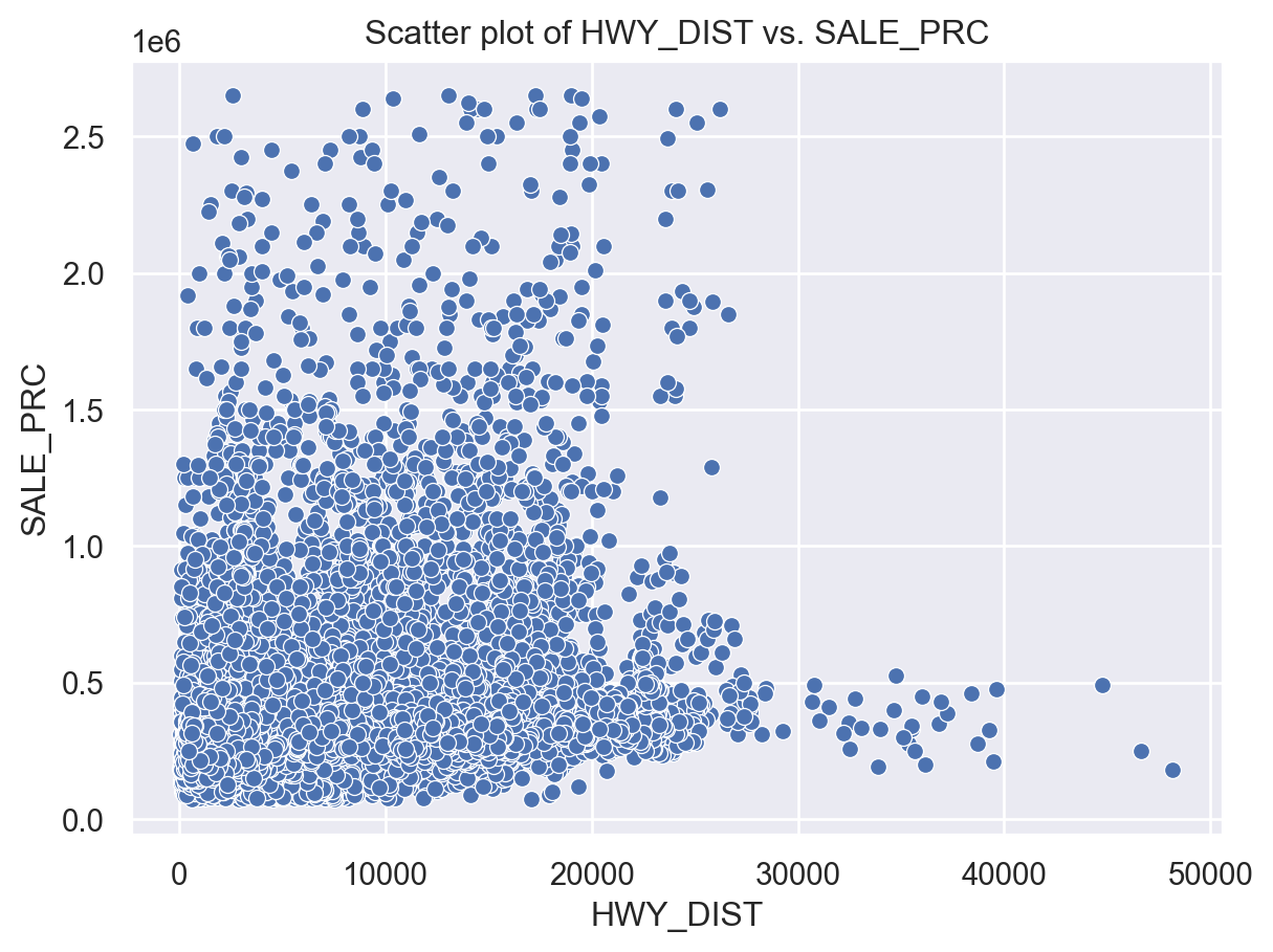

sns.histplot(df['RAIL_DIST'], bins=30, kde=True)
plt.title('Distribution of RAIL_DIST')
plt.show()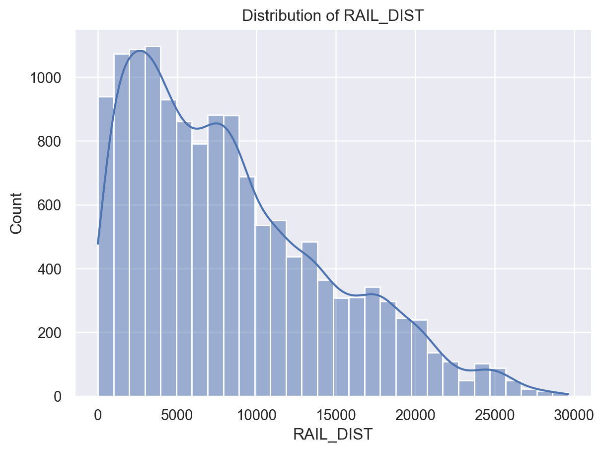

features = ['LATITUDE', 'LONGITUDE', 'LND_SQFOOT', 'TOT_LVG_AREA', 'SPEC_FEAT_VAL', 'RAIL_DIST', 'OCEAN_DIST', 'WATER_DIST', 'CNTR_DIST', 'SUBCNTR_DI', 'HWY_DIST', 'age', 'avno60plus', 'month_sold', 'structure_quality']
target = 'SALE_PRC'

df = pd.read_csv('miami-housing.csv')
X = df[features]
y = df[target]

correlation_matrix = df[features + [target]].corr()
plt.figure(figsize=(10, 6))
sns.heatmap(correlation_matrix,  cmap="coolwarm", fmt=".2f")
for i in range(len(correlation_matrix)):
    for j in range(len(correlation_matrix)):
        plt.text(j + 0.5, i + 0.5, f"{correlation_matrix.iloc[i, j]:.2f}", ha='center', va='center', fontsize=10)
plt.title("Correlation Heatmap")
plt.show()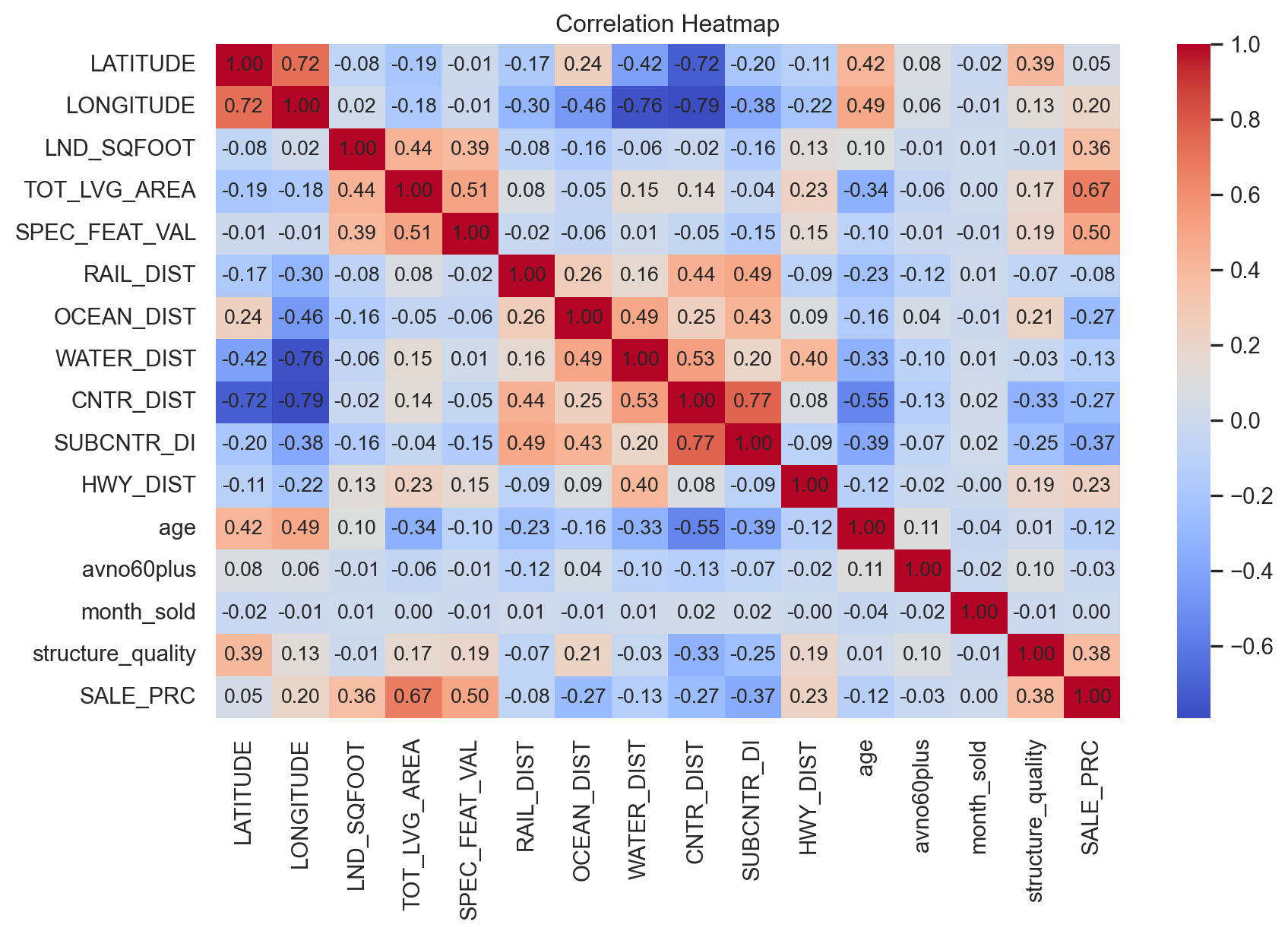

sns.histplot(df[target], kde=True)
plt.title("Distribution of Sale Price")
plt.xlabel("Sale Price")
plt.show()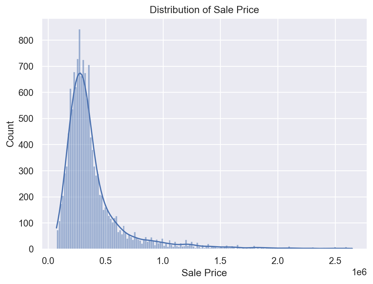

X_train, X_test, y_train, y_test = train_test_split(X, y, test_size=0.2)
gb_model = GradientBoostingRegressor(n_estimators=100, learning_rate=0.1, max_depth=3)
model = gb_model.fit(X_train, y_train)
y_pred = model.predict(X_test)
r2_score(y_pred,y_test)

0.8851074423455013

fea_importances = model.feature_importances_

fea_importance_df = pd.DataFrame({'Feature': features, 'Importance': fea_importances})

fea_importance_df = fea_importance_df.sort_values(by='Importance', ascending=False)

plt.barh(fea_importance_df['Feature'], fea_importance_df['Importance'])
plt.xlabel('Importance')
plt.title('Feature Importance')
plt.show()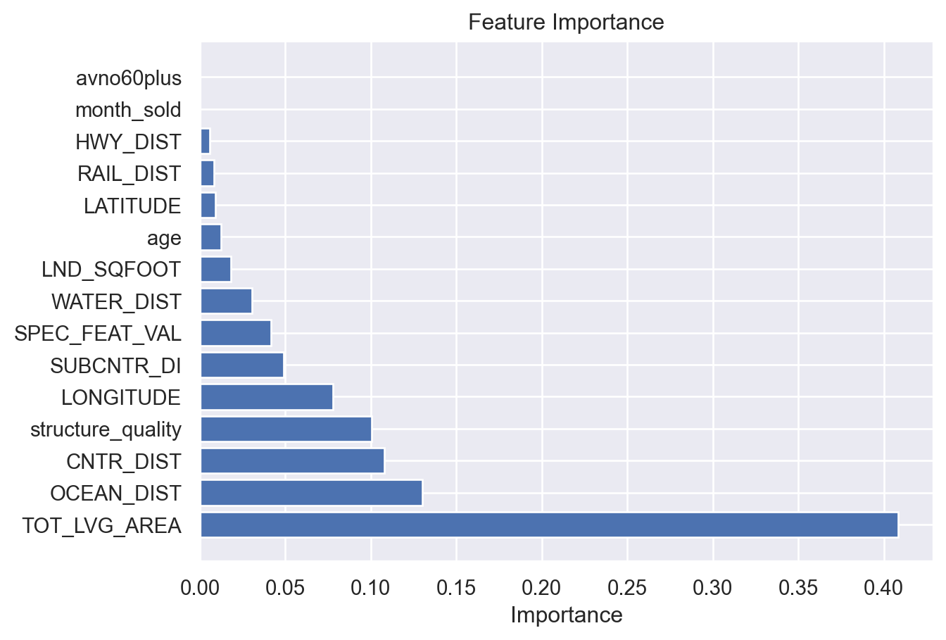

%matplotlib inline
import numpy as np
import pandas as pd
import matplotlib.pyplot as plt
from sklearn.preprocessing import PolynomialFeatures
from sklearn.linear_model import LinearRegression
chosen_feature = 'LATITUDE'
y = df['SALE_PRC']
poly_features = PolynomialFeatures(degree=2, include_bias=False)
X_poly = poly_features.fit_transform(X[[chosen_feature]])
lin_reg = LinearRegression()
lin_reg.fit(X_poly, y)
plt.scatter(X[chosen_feature], y, color='r', label='Original Data')
X_line = np.linspace(X[chosen_feature].min(), X[chosen_feature].max(), 100).reshape(-1, 1)
X_line_poly = poly_features.transform(X_line)
y_line_pred = lin_reg.predict(X_line_poly)
plt.plot(X_line, y_line_pred, color='b', label='Polynomial Regression')
plt.xlabel(chosen_feature)
plt.ylabel('SALE_PRC')
plt.legend()
plt.show()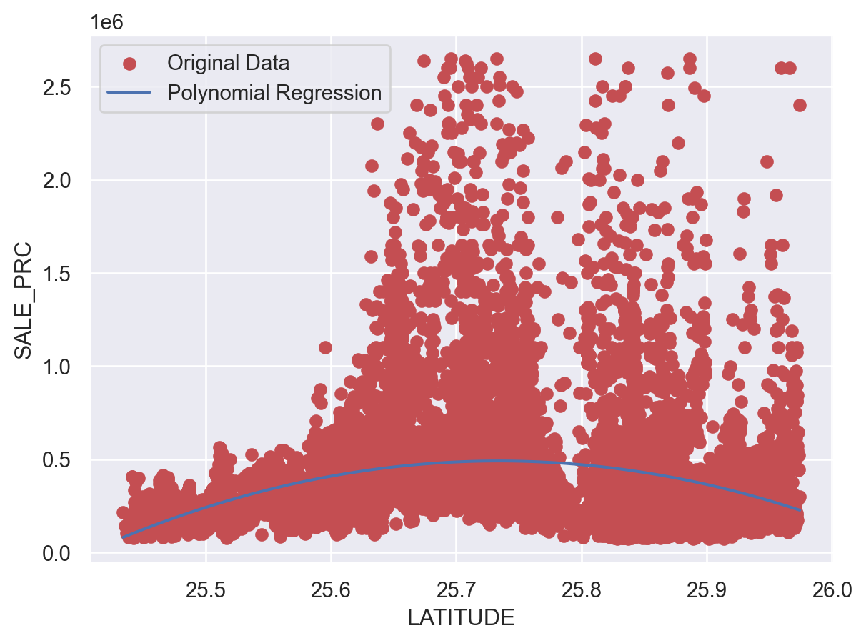

from sklearn.model_selection import train_test_split
X_train,X_test,y_train,y_test=train_test_split(X,y,test_size=0.2,random_state=42)

from sklearn.linear_model import LinearRegression

y = df['SALE_PRC']
num_features = X.shape[1]
fig, axes = plt.subplots(nrows=num_features, ncols=1, figsize=(10, 2*num_features))

for i, feature in enumerate(X.columns):
    X_single_feature = X[feature].values.reshape(-1, 1)
    lin_reg = LinearRegression()
    lin_reg.fit(X_single_feature, y)
    axes[i].scatter(X[feature], y, color='r', label='Original Data')
    X_line = np.linspace(X[feature].min(), X[feature].max(), 100).reshape(-1, 1)
    y_line_pred = lin_reg.predict(X_line)
    axes[i].plot(X_line, y_line_pred, color='b', label='Simple Linear Regression')
    axes[i].set_xlabel(feature)
    axes[i].set_ylabel('SALE_PRC')
    axes[i].legend()
plt.show()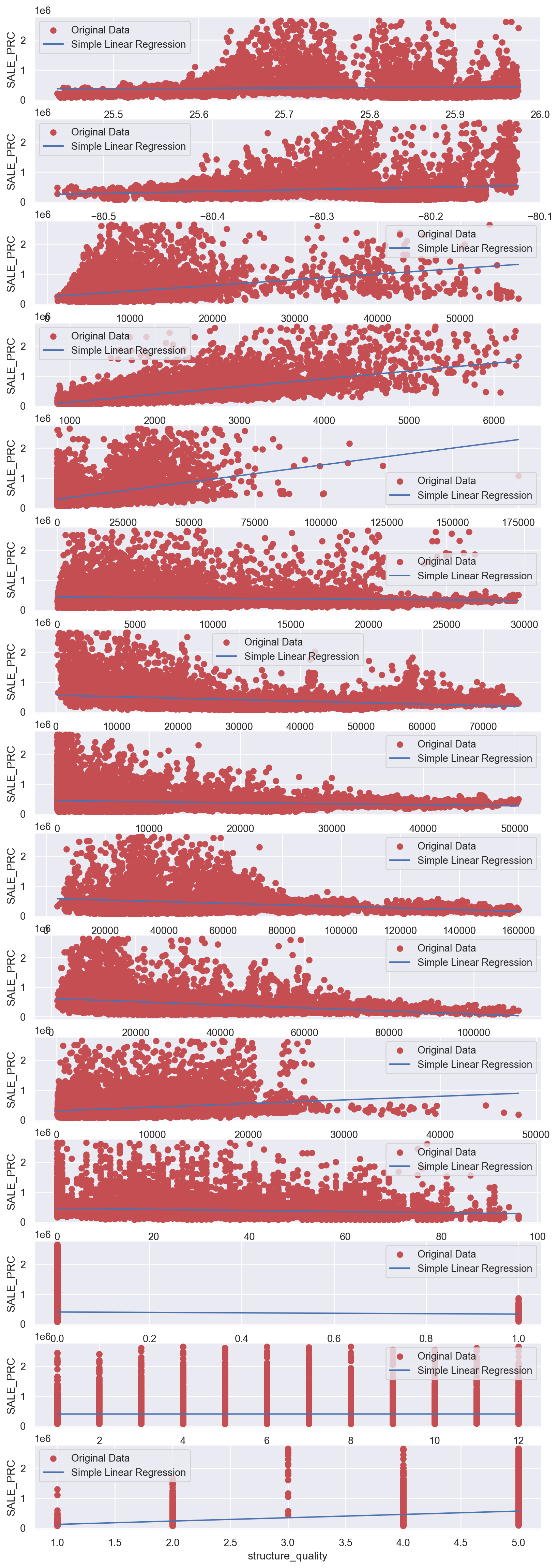

poly_features = PolynomialFeatures(degree=2, include_bias=False)
X_poly = poly_features.fit_transform(X)
X_train, X_test, y_train, y_test = train_test_split(X_poly, y, test_size=0.2, random_state=42)
poly_reg_model = LinearRegression()
poly_reg_model.fit(X_train, y_train)
accuracy = poly_reg_model.score(X_test, y_test)
print(f"Polynomial Regression Model Accuracy: {accuracy}")

Polynomial Regression Model Accuracy: 0.881111708167996

X_poly.round(2)

array([[ 2.589e+01, -8.016e+01,  9.375e+03, ...,  6.400e+01,  3.200e+01,
         1.600e+01],
       [ 2.589e+01, -8.015e+01,  9.375e+03, ...,  8.100e+01,  3.600e+01,
         1.600e+01],
       [ 2.589e+01, -8.015e+01,  9.375e+03, ...,  4.000e+00,  8.000e+00,
         1.600e+01],
       ...,
       [ 2.578e+01, -8.026e+01,  8.460e+03, ...,  4.900e+01,  2.800e+01,
         1.600e+01],
       [ 2.578e+01, -8.026e+01,  7.500e+03, ...,  6.400e+01,  3.200e+01,
         1.600e+01],
       [ 2.578e+01, -8.026e+01,  8.833e+03, ...,  1.210e+02,  4.400e+01,
         1.600e+01]])

print(poly_reg_model.coef_.round(2))

[ 1.64638752e+09  1.43501940e+08  1.99361000e+03  7.18771000e+03
  5.72473000e+03  1.09326100e+04 -2.20423400e+04 -2.27902000e+03
  5.99300000e+01 -8.40520000e+02 -1.25848900e+04 -1.22307374e+06
 -1.67500006e+06 -1.76007415e+06  2.15822777e+07  4.92283607e+06
  2.37884737e+07 -7.24700000e+01 -2.26910000e+02 -2.41000000e+01
 -6.05400000e+01  7.95200000e+01  8.66300000e+01  5.84100000e+01
 -5.57000000e+00  4.27100000e+01  9.13476000e+03  1.16614383e+07
 -2.10318000e+03 -8.07204800e+04  4.66524507e+06  1.23000000e+00
  1.33300000e+01  6.36000000e+01  1.16820000e+02 -2.49730000e+02
 -2.30000000e-01  1.92500000e+01 -1.20200000e+01 -1.43320000e+02
 -1.23242000e+04  3.73434037e+06 -2.26988600e+04  2.44413360e+05
 -0.00000000e+00 -0.00000000e+00  0.00000000e+00  0.00000000e+00
  0.00000000e+00  0.00000000e+00 -0.00000000e+00  0.00000000e+00
  0.00000000e+00  1.00000000e-01 -2.84000000e+00  3.00000000e-02
 -3.70000000e-01  1.00000000e-02  0.00000000e+00 -0.00000000e+00
 -0.00000000e+00  0.00000000e+00 -0.00000000e+00  0.00000000e+00
  0.00000000e+00 -2.56000000e+00 -8.56900000e+01 -1.20000000e-01
  2.69200000e+01 -0.00000000e+00  0.00000000e+00  0.00000000e+00
 -0.00000000e+00  0.00000000e+00 -0.00000000e+00  0.00000000e+00
 -4.00000000e-02 -2.83000000e+00  1.00000000e-02  3.50000000e-01
 -0.00000000e+00  0.00000000e+00  0.00000000e+00 -0.00000000e+00
  0.00000000e+00 -0.00000000e+00  1.00000000e-02  4.45000000e+00
  3.00000000e-02  1.29000000e+00 -0.00000000e+00 -0.00000000e+00
 -0.00000000e+00  0.00000000e+00 -0.00000000e+00 -6.00000000e-02
 -1.37300000e+01  3.00000000e-02  6.00000000e-02 -0.00000000e+00
  0.00000000e+00 -0.00000000e+00  0.00000000e+00  8.00000000e-02
  4.09000000e+00  1.00000000e-02  7.20000000e-01 -0.00000000e+00
  0.00000000e+00 -0.00000000e+00 -1.00000000e-02  4.62000000e+01
 -8.00000000e-02 -6.50000000e-01  0.00000000e+00  0.00000000e+00
  3.00000000e-02 -3.48700000e+01  5.00000000e-02  1.60000000e-01
  0.00000000e+00  4.00000000e-02 -1.87100000e+01 -7.00000000e-02
  1.34000000e+00  9.35000000e+00  6.75860000e+02 -1.79900000e+01
  1.14010000e+02  5.66658400e+05  1.42371000e+03 -2.88494500e+04
 -1.58070000e+02 -8.33910000e+02  1.79120600e+04]

print(poly_reg_model.intercept_)

-15030137122.62008

degree = 2
fig, axes = plt.subplots(nrows=num_features, ncols=1, figsize=(10, 2*num_features))
fig.tight_layout(h_pad=4)
for i, feature in enumerate(X.columns):
    X_single_feature = X[feature].values.reshape(-1, 1)
    poly_features = PolynomialFeatures(degree=degree, include_bias=False)
    X_poly = poly_features.fit_transform(X_single_feature)
    poly_reg = LinearRegression()
    poly_reg.fit(X_poly, y)
    axes[i].scatter(X[feature], y, color='r', label='Original Data')
    X_line = np.linspace(X[feature].min(), X[feature].max(), 100).reshape(-1, 1)
    X_line_poly = poly_features.transform(X_line)
    y_line_pred = poly_reg.predict(X_line_poly)
    axes[i].plot(X_line, y_line_pred, color='b', label=f'Polynomial Regression (Degree {degree})')
    axes[i].set_xlabel(feature)
    axes[i].set_ylabel('SALE_PRC')
    axes[i].legend()

plt.show()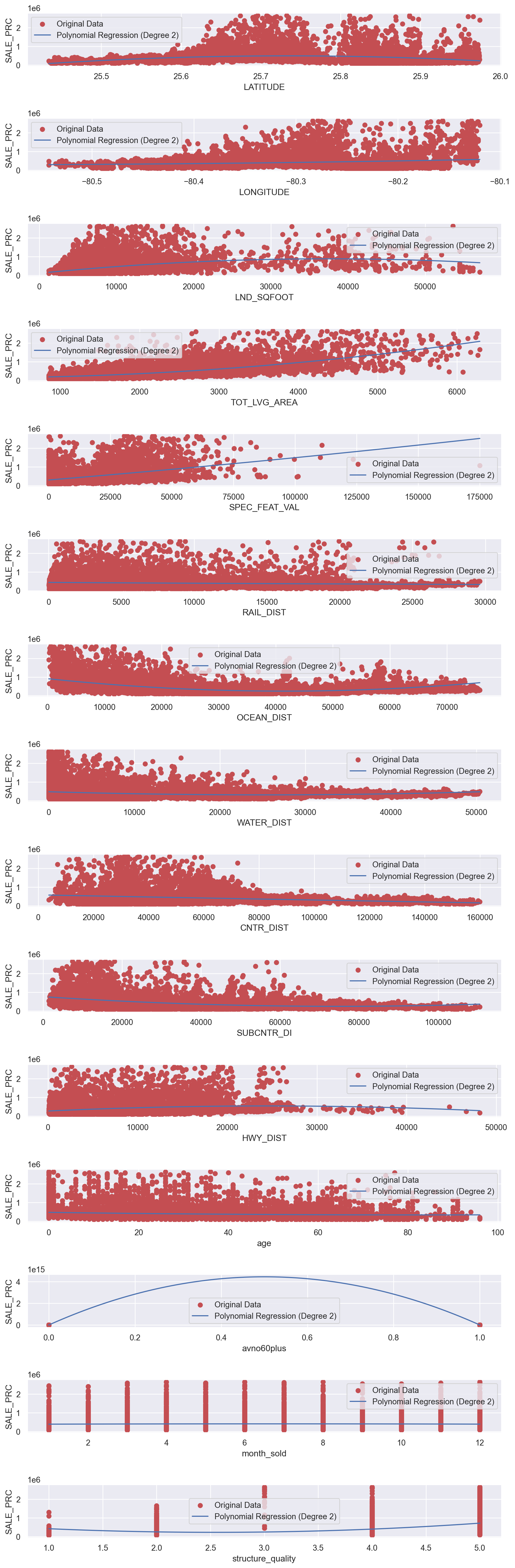

poly_features = PolynomialFeatures(degree=2, include_bias=False)
X_poly = poly_features.fit_transform(X)
X_train, X_test, y_train, y_test = train_test_split(X_poly, y, test_size=0.2, random_state=42)
poly_reg_model = LinearRegression()
poly_reg_model.fit(X_train, y_train)
accuracy = poly_reg_model.score(X_test, y_test)
print(f"Polynomial Regression Model Accuracy: {accuracy}")

Polynomial Regression Model Accuracy: 0.881111708167996

num_features = X.shape[1]
degree = 3
fig, axes = plt.subplots(nrows=num_features, ncols=1, figsize=(10, 2*num_features))
fig.tight_layout(h_pad=4)
for i, feature in enumerate(X.columns):
    X_single_feature = X[feature].values.reshape(-1, 1)
    poly_features = PolynomialFeatures(degree=degree, include_bias=True) 
    X_poly = poly_features.fit_transform(X_single_feature)
    poly_reg = LinearRegression()
    poly_reg.fit(X_poly, y)
    axes[i].scatter(X[feature], y, color='r', label='Original Data')
    X_line = np.linspace(X[feature].min(), X[feature].max(), 100).reshape(-1, 1)
    X_line_poly = poly_features.transform(X_line)
    y_line_pred = poly_reg.predict(X_line_poly)
    axes[i].plot(X_line, y_line_pred, color='b', label=f'Polynomial Regression (Degree {degree})')
    axes[i].set_xlabel(feature)
    axes[i].set_ylabel('SALE_PRC')
    axes[i].legend()
plt.show()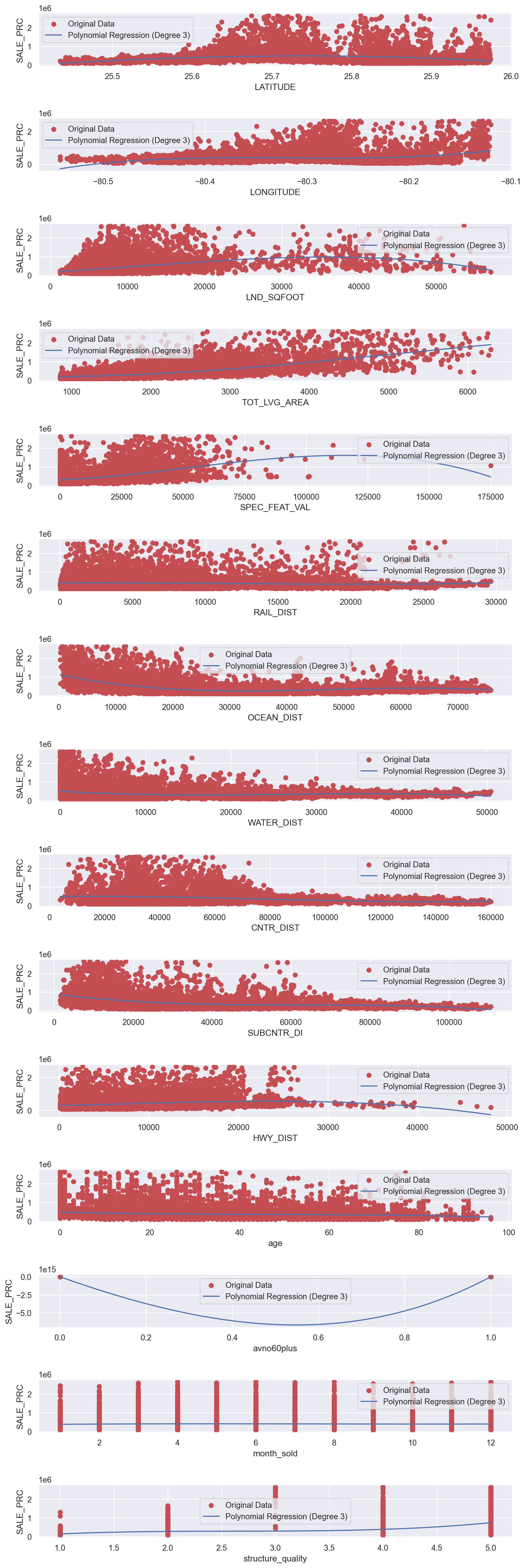

from sklearn.preprocessing import PolynomialFeatures
X = df[features]
degree = 3
poly_features = PolynomialFeatures(degree=degree, include_bias=False)
X_poly = poly_features.fit_transform(X)
poly_feature = poly_features.get_feature_names_out(X.columns)
X_poly_df = pd.DataFrame(X_poly, columns=poly_feature)
print(X_poly_df.head())

    LATITUDE  LONGITUDE  LND_SQFOOT  TOT_LVG_AREA  SPEC_FEAT_VAL  RAIL_DIST  \
0  25.891031 -80.160561      9375.0        1753.0            0.0     2815.9   
1  25.891324 -80.153968      9375.0        1715.0            0.0     4359.1   
2  25.891334 -80.153740      9375.0        2276.0        49206.0     4412.9   
3  25.891765 -80.152657     12450.0        2058.0        10033.0     4585.0   
4  25.891825 -80.154639     12800.0        1684.0        16681.0     4063.4   

   OCEAN_DIST  WATER_DIST  CNTR_DIST  SUBCNTR_DI  ...  avno60plus^3  \
0     12811.4       347.6    42815.3     37742.2  ...           0.0   
1     10648.4       337.8    43504.9     37340.5  ...           0.0   
2     10574.1       297.1    43530.4     37328.7  ...           0.0   
3     10156.5         0.0    43797.5     37423.2  ...           0.0   
4     10836.8       326.6    43599.7     37550.8  ...           0.0   

   avno60plus^2 month_sold  avno60plus^2 structure_quality  \
0                      0.0                             0.0   
1                      0.0                             0.0   
2                      0.0                             0.0   
3                      0.0                             0.0   
4                      0.0                             0.0   

   avno60plus month_sold^2  avno60plus month_sold structure_quality  \
0                      0.0                                      0.0   
1                      0.0                                      0.0   
2                      0.0                                      0.0   
3                      0.0                                      0.0   
4                      0.0                                      0.0   

   avno60plus structure_quality^2  month_sold^3  \
0                             0.0         512.0   
1                             0.0         729.0   
2                             0.0           8.0   
3                             0.0         729.0   
4                             0.0         343.0   

   month_sold^2 structure_quality  month_sold structure_quality^2  \
0                           256.0                           128.0   
1                           324.0                           144.0   
2                            16.0                            32.0   
3                           324.0                           144.0   
4                           196.0                           112.0   

   structure_quality^3  
0                 64.0  
1                 64.0  
2                 64.0  
3                 64.0  
4                 64.0  

[5 rows x 815 columns]

from sklearn.preprocessing import StandardScaler, LabelEncoder
from sklearn.metrics import confusion_matrix, roc_auc_score
import lightgbm as lgb
import xgboost as xgb
from datetime import datetime

df = pd.read_csv('miami-housing.csv')
thresholdPrice = 500000
df['Above_Threshold'] = (df['SALE_PRC'] > thresholdPrice).astype(int)
df = df.drop(['PARCELNO'], axis=1)
y = df['Above_Threshold'].values
labelencoder = LabelEncoder()
Y = labelencoder.fit_transform(y)   
X = df.drop(labels=['Above_Threshold', 'SALE_PRC'], axis=1)  
feature_names = np.array(X.columns)
scaler = StandardScaler()
scaler.fit(X)
X = scaler.transform(X)
X_train, X_test, y_train, y_test = train_test_split(X, Y, test_size=0.2, random_state=42)

dtrain_lgb = lgb.Dataset(X_train, label=y_train)

lgbm_params = {
    'learning_rate': 0.05,
    'boosting_type': 'gbdt',
    'objective': 'binary',
    'metric': ['auc', 'binary_logloss'],
    'num_leaves': 100,
    'max_depth': 10
}
startLgb = datetime.now()
clf_lgb = lgb.train(lgbm_params, dtrain_lgb, 50)
stopLgb = datetime.now()
executionTime_lgb = stopLgb - startLgb
ypred_lgb = clf_lgb.predict(X_test)
ypred_lgb = (ypred_lgb >= 0.5).astype(int)
dtrain_xgb = xgb.DMatrix(X_train, label=y_train)
parameters_xgb = {
    'max_depth': 10,
    'objective': 'binary:logistic',
    'eval_metric': 'auc',
    'learning_rate': 0.05
}
startXgb = datetime.now()
xg = xgb.train(parameters_xgb, dtrain_xgb, 50)
stopXgb = datetime.now()
executionTime_xgb = stopXgb - startXgb
dtest_xgb = xgb.DMatrix(X_test)
ypred_xgb = xg.predict(dtest_xgb)
ypred_xgb = (ypred_xgb >= 0.5).astype(int)
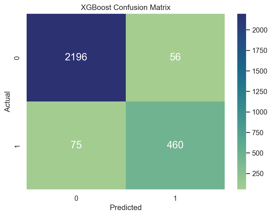
cm_xgb = confusion_matrix(y_test, ypred_xgb)
sns.heatmap(cm_xgb,fmt='g',cmap="crest" )
for i in range(len(cm_xgb)):
    for j in range(len(cm_xgb[0])):
        plt.text(j + 0.5, i + 0.5, str(cm_xgb[i, j]), ha='center', va='center', fontsize=16, color='white')
plt.xlabel('Predicted')
plt.ylabel('Actual')
plt.title('XGBoost Confusion Matrix')
plt.show() 
print("_________________________________________________")
print("LGBM execution time is: ", executionTime_lgb )
print("XGBoost execution time is: ", executionTime_xgb)
print("_________________________________________________")
print("Accuracy with LGBM = ", np.mean(ypred_lgb == y_test))
print("Accuracy with XGBoost = ", np.mean(ypred_xgb == y_test))
print("___________________________________________________")
print("AUC score with LGBM is: ", roc_auc_score(y_test, ypred_lgb))
print("AUC score with XGBoost is: ", roc_auc_score(y_test,ypred_xgb))

[LightGBM] [Info] Number of positive: 2015, number of negative: 9130
[LightGBM] [Info] Auto-choosing col-wise multi-threading, the overhead of testing was 0.000390 seconds.
You can set `force_col_wise=true` to remove the overhead.
[LightGBM] [Info] Total Bins 2921
[LightGBM] [Info] Number of data points in the train set: 11145, number of used features: 15
[LightGBM] [Info] [binary:BoostFromScore]: pavg=0.180799 -> initscore=-1.510946
[LightGBM] [Info] Start training from score -1.510946
_________________________________________________
LGBM execution time is:  0:00:00.094721
XGBoost execution time is:  0:00:00.178523
_________________________________________________
Accuracy with LGBM =  0.9551489056332975
Accuracy with XGBoost =  0.9529960531036957
___________________________________________________
AUC score with LGBM is:  0.9180927441443535
AUC score with XGBoost is:  0.9174731495161104